Induced Triploidy Does Not Alter Per-Genome Ribosomal DNA Copy Number in the Pacific Oyster Magallana gigas
A short non-peer-reviewed scientific report
This report is a Roberts Lab working manuscript. It has not been peer reviewed.
It is shared to make small scientific efforts, preliminary analyses, technical observations, and exploratory work openly available.
1 Abstract
Chemically induced triploidy is used commercially in the Pacific oyster (Magallana gigas, formerly Crassostrea gigas) to suppress reproductive investment, but its consequences for the ribosomal DNA (rDNA) arrays — the multi-copy loci that set the ceiling on ribosome biogenesis — are unknown. We estimated 45S and 5S rDNA copy number per haploid genome from whole-genome shotgun sequencing of 32 animals drawn from two families (F05 and F14), sampled as 16 labelled diploids and 16 labelled induced triploids. Because copy-number estimation depends on the ploidy assignment, we verified ploidy directly from the sequence data using B-allele frequencies at heterozygous sites in 5,000 uniquely mappable single-copy windows, calibrated per animal against simulations built on that animal’s own depth distribution. The ploidy index was sharply bimodal with an empty separating band, and 6 of 32 animals contradicted their induction label — one labelled diploid read triploid and five labelled triploids read diploid — so all analyses were run twice, on ploidy as labelled (the pre-registered contrast) and on ploidy as measured. Triploidy did not detectably change 45S rDNA dosage per haploid genome under either assignment (0.95-fold, 95% CI 0.80–1.13, p = 0.33 as labelled; 0.89-fold, 95% CI 0.75–1.05, p = 0.07 as measured), and the three transcribed subunits agreed. 5S copy number likewise did not track ploidy but differed strongly between families (p = 2e-04; means 75 copies in F05 against 113 in F14). Mitogenome copies per haploid nuclear genome fell by 0.73-fold in triploids (95% CI 0.57–0.92, p = 0.015), exactly the two-thirds dilution expected if mitochondrial content per cell is set independently of nuclear ploidy; re-expressed per cell the difference vanished, providing corroboration of the ploidy calls from a signal independent of allele balance. An exploratory scan of 25,038 1-kb windows overlapping 10,610 protein-coding genes found no locus associated with ploidy but 572 associated with family, enriched for innate-immunity and cell-adhesion genes. Induced triploidy in these animals scales the genome without redistributing rDNA or gene-level dosage; the dominant axis of copy-number variation is family background, not ploidy.
Keywords. Magallana gigas, induced triploidy, ribosomal DNA, copy number variation, B-allele frequency, ploidy verification
2 Background
The 45S rDNA arrays encode the 18S, 5.8S and 28S ribosomal RNAs as tandem repeats, and the 5S arrays encode the 5S rRNA separately. Copy number at these loci varies widely within species and is not fixed developmentally, which makes it a candidate mediator of any change in growth or stress physiology that follows a change in genome dosage.
Induced triploidy adds a third nuclear genome copy without altering the per-genome sequence content, so the naive expectation is that copy number per haploid genome is unchanged and copy number per cell rises by half. That expectation is not guaranteed. Triploid induction acts by blocking a meiotic division, and the resulting genomes are assembled from a maternal complement that has not been reduced; if rDNA arrays differ systematically between the retained and the reduced complements, or if array size is subject to selection during the disturbed early divisions, per-genome dosage could shift.
Testing this requires knowing which animals are actually triploid. Induction is incomplete in practice, and the ploidy recorded at the hatchery is a record of treatment, not of outcome. We therefore treated ploidy verification as part of the measurement rather than as metadata, and determined it from the same sequence data used for copy number.
This study addresses three questions: (i) does 45S rDNA copy number per haploid genome differ between diploid and induced-triploid animals; (ii) does 5S rDNA copy number; and (iii) how much of the variation in either is attributable to family background rather than ploidy.
3 Methods
3.1 Animals and design
32 animals from a USDA-NRSP-8 Pacific oyster breeding programme were analysed, comprising two families (F05, F14) crossed with two induction treatments, 8 animals per family per treatment (32 total, a balanced 2 x 2 design as labelled). Sample identifiers encode family, labelled ploidy and animal number as F<family><ploidy>n<animal>; for example F052n03 is family F05, labelled 2n, animal 3, and F143n07 is family F14, labelled 3n, animal 7. Ploidy labels reflect the induction treatment applied at the hatchery, not a cytometric measurement. Animal husbandry, spawning and triploid induction were performed by the source programme and are outside the scope of this analysis; the induction agent, dose and timing are not documented in the material available to us, and this limits interpretation of the induction failures reported below.
3.2 Sequencing
Whole-genome shotgun paired-end libraries were sequenced for all 32 animals, yielding 3.3 billion read pairs in total (84–130 million reads per animal) at 2 x 150 bp. Library preparation chemistry, instrument model and run configuration are not recorded in the project metadata available to this analysis; the read group written by the pipeline records platform ILLUMINA only. Post-trimming read length was 149 bp and Q30 base fraction 89.8–92.0%. Observed GC content was 33.8–37.6%.
3.3 Raw data and output locations
All primary and derived data reside on the laboratory analysis server raven (raven.fish.washington.edu) under the project root
/home/shared/8TB_HDD_03/mattgeorgephd/USDA-NRSP-8-gigas-rDNAreferred to below as $D. Contents relevant to reproduction:
| path | contents |
|---|---|
$D/data/raw/<sample>_R{1,2}_001.fastq.gz |
raw paired FASTQ, 64 files, 245 GB total |
$D/data/raw/checksums.md5, checksums_full.md5 |
MD5 manifests for the raw FASTQ set |
$D/data/genomes/cassette_reference.fna |
alignment reference, 571 MB, 32 contigs, with BWA index |
$D/data/genomes/assembly_report.txt |
NCBI assembly report for the source assembly |
$D/reference/single_copy_windows.bed |
5,000 single-copy control windows |
$D/reference/gc_calibration_windows.bed |
24,605 GC-stratified calibration windows |
$D/reference/array_mask.bed |
coordinates of the masked tandem rDNA arrays |
$D/reference/mappability.bw, mappability/ |
GenMap mappability track used for window selection |
$D/analysis/<sample>/ |
per-sample pipeline outputs, 32 directories, 62 MB total |
$D/code/rdna_pipeline.sh |
the per-sample pipeline, verbatim as executed |
$D/work/<sample>/ |
scratch; BAMs deleted after depth extraction unless --keep-bam |
Per-sample outputs in $D/analysis/<sample>/ comprise <sample>.baf.tsv.gz (allele depths at biallelic SNP sites), <sample>.control_windows.depth.tsv.gz and <sample>.gc_calibration.depth.tsv.gz (1-kb mean depths), <sample>.cassette.depth.Q20.tsv.gz (per-base depth on the cassette contigs), <sample>.cassette_mapq.txt, <sample>.fastp.json/.html/.log, <sample>.flagstat.txt, <sample>.idxstats.txt, <sample>.samstats.txt, <sample>.markdup.json and <sample>.bwa.log.
Alignments were not retained: BAMs are deleted at the end of each sample to bound disk use, so reproducing any BAM-level analysis requires realignment from FASTQ (approximately 4 h per sample at 11 threads). At the time of writing two BAMs (F052n01, F053n01) remain in $D/work/ from pilot runs.
3.4 Reference construction
Reads were aligned to a composite reference built from the NCBI RefSeq assembly GCF_963853765.1 (xbMagGiga1.1, Magallana gigas, taxon 29159; annotation release GCF_963853765.1-RS_2024_06, 20 June 2024) (National Center for Biotechnology Information 2024). The assembly comprises 10 chromosomes (563.19 Mb) and 19 unplaced scaffolds (0.80 Mb), 563.99 Mb in total.
Tandem rDNA arrays cannot be quantified by depth in an assembly that collapses them, and reads from the arrays otherwise scatter across the collapsed copies. The reference was therefore modified in two coordinated steps:
- Array masking. The assembled tandem arrays were hard-masked (replaced by N), namely the 45S array at
NC_088862.1:1–65,425(chromosome 10) and the 5S array atNC_088857.1:44,123,955–44,205,662(chromosome 5). Coordinates are in$D/reference/array_mask.bed. - Single-monomer contigs appended. One full repeat period of each array was appended as a separate contig, so that all array-derived reads compete for a single unambiguous target and depth over that contig is proportional to array size:
rDNA_45S_monomer, 11,764 bp, fromNC_088862.1:6,284–18,047, containing 18S–ITS1–5.8S–ITS2–28S–IGS;rDNA_5S_monomer, 1,670 bp, fromNC_088857.1:44,124,662–44,126,331, containing the 5S gene and its spacer.
The mitogenome (NC_001276.1, 18,224 bp) was appended as a third extra contig. The final reference contains 32 sequences. Feature coordinates within the monomers are in $D/reference/rDNA_45S_monomer_features.bed and rDNA_5S_monomer_features.bed:
| contig | feature | coordinates (0-based, half-open) |
|---|---|---|
rDNA_45S_monomer |
28S rRNA | 0–3,782 |
rDNA_45S_monomer |
5.8S rRNA | 4,345–4,499 |
rDNA_45S_monomer |
18S rRNA | 4,954–6,775 |
rDNA_45S_monomer |
transcribed unit (primary target) | 0–6,775 |
rDNA_45S_monomer |
IGS | 6,775–11,764 |
rDNA_5S_monomer |
5S rRNA (primary target) | 0–119 |
rDNA_5S_monomer |
5S spacer | 119–1,670 |
The IGS was flagged as repeat-contaminated during reference construction and its copy number is reported but not interpreted. Masking was verified per sample by a MAPQ histogram of reads aligning to each appended contig (<sample>.cassette_mapq.txt); the check confirms that the masking still forces array reads to map uniquely to the monomer.
Control windows. Copy number requires a single-copy depth reference. 5,000 1-kb windows were selected genome-wide on two criteria: perfect mappability in the GenMap track (Pockrandt et al. 2020) (minimum mappability 1.0 across the window) and depth consistent with single-copy status. Because these windows follow the genome’s own GC distribution they are nearly empty above 55% GC, which is exactly where the 45S cassette sits (51–56% GC); a second set of 24,605 GC-stratified calibration windows was therefore built to populate the high-GC range. Both sets are used together as the denominator pool; using the single-copy set alone shifts the high-GC denominator and inflates 28S and 5.8S copy number by approximately 17%.
3.5 Read processing and alignment
The complete per-sample pipeline is $D/code/rdna_pipeline.sh, invoked as rdna_pipeline.sh <SAMPLE_ID> [--keep-bam] with THREADS set by environment variable (11 for the production batch, run four samples at a time on a 48-core host). Every stage is skipped if its output exists, so interrupted samples resume without realignment.
Adapter and quality trimming with fastp (Chen 2023):
fastp -i $R1 -I $R2 -o ${SM}_R1.trim.fastq.gz -O ${SM}_R2.trim.fastq.gz \
  --detect_adapter_for_pe --cut_front --cut_tail --cut_mean_quality 20 \
  --qualified_quality_phred 20 --unqualified_percent_limit 40 --length_required 50 \
  --thread 16 --json ${SM}.fastp.json --html ${SM}.fastp.html
Alignment with BWA-MEM (Li and Durbin 2009), coordinate sorting and duplicate marking with SAMtools (Danecek et al. 2021) in a single stream:
bwa mem -t $THREADS -R "@RG\tID:${SM}\tSM:${SM}\tPL:ILLUMINA\tLB:${SM}" \
    $REF ${SM}_R1.trim.fastq.gz ${SM}_R2.trim.fastq.gz \
  | samtools fixmate -m -u -@ 4 - - \
  | samtools sort -u -@ 8 -m 2G -T sorttmp - \
  | samtools markdup -@ 4 --json -f ${SM}.markdup.json - ${SM}.bam
samtools index -@ 8 ${SM}.bam
Duplicates are marked, not removed; they are excluded downstream by samtools depth, which by default filters UNMAP,SECONDARY,QCFAIL,DUP. This default was deliberately not overridden: retaining duplicates would inflate depth non-uniformly between the cassette and the control windows.
3.6 Depth extraction
Per-base depth was extracted at matched stringency (MAPQ >= 20, base quality >= 20) over three target sets and aggregated to 1-kb window means for the genomic sets:
samtools depth -a -b single_copy_windows.bed   -Q 20 -q 20 $BAM | agg1kb | gzip > control_windows.depth.tsv.gz
samtools depth -a -b gc_calibration_windows.bed -Q 20 -q 20 $BAM | agg1kb | gzip > gc_calibration.depth.tsv.gz
samtools depth -a -b cassette_contigs.bed       -Q 20 -q 20 $BAM | gzip        > cassette.depth.Q20.tsv.gz
where agg1kb is awk '{k=$1"\t"int(($2-1)/1000)*1000; s[k]+=$3; n[k]++} END{for(k in s) print k, s[k]/n[k], n[k]}' followed by a coordinate sort. Aggregation is exact because every window in both BED files begins on a 1-kb boundary. The window files carry four columns — chromosome, start, mean depth, window length — and the fourth column is a length, not an end coordinate; reading it as a coordinate silently sets every depth to 1000.
The cassette file retains per-base resolution so that arbitrary sub-features of the monomers can be quantified without realignment.
3.7 Copy-number estimation
Copy number for a feature is the ratio of its mean depth to the depth expected from a single diploid-equivalent locus, both measured at the same stringency:
\[ \mathrm{CN}_{\text{feature}} = \frac{\bar{d}_{\text{feature}}}{d_{1\times}(\mathrm{GC}_{\text{feature}})} \]
The denominator \(d_{1\times}\) is estimated empirically by GC matching rather than from a fitted genome-wide GC–depth curve. For a feature of GC content \(g\), control windows with GC in \([g - 0.04, g + 0.04]\) are selected from the pooled single-copy and GC-calibration sets, the window is widened in 0.01 steps until at least 300 windows are available, and the denominator is the median depth of the matched windows. A fitted curve is not used because depth is flat across GC within the cassette, so the genomic curve — driven by rare high-GC windows — is not transferable to it. Confidence limits on copy number come from 400 bootstrap resamples of the matched window set (2.5th and 97.5th percentiles of the bootstrap median), propagated as \(\mathrm{CN}_{lo} = \bar{d} / d_{97.5}\) and \(\mathrm{CN}_{hi} = \bar{d} / d_{2.5}\).
Copy number so defined is per haploid genome, because the denominator is the depth of a locus present once per haploid complement. Multiplying by ploidy gives copies per cell.
3.8 Ploidy determination
Ploidy was determined from allele balance at heterozygous sites, independently of the induction label. At a heterozygous site a diploid yields a B-allele fraction (BAF) centred on 1/2, whereas a triploid carries either one or two copies of the alternate allele and yields fractions centred on 1/3 and 2/3. At the coverage realised here these components are not separable by eye, so the statistic is calibrated by simulation per animal (Figure 1).
Variant calling. Restricted to the 5,000 uniquely mappable single-copy control windows, because unique mappability is the precondition for BAF-based ploidy: paralogous mapping manufactures false intermediate allele fractions. Same duplicate, MAPQ and base-quality filtering as the depth step, using BCFtools (Danecek et al. 2021):
bcftools mpileup -f $REF -R single_copy_windows.bed -q 20 -Q 20 -I -a AD,DP -d 200 -Ou $BAM \
  | bcftools call -m -v -Ou \
  | bcftools view -m2 -M2 -v snps -Ou \
  | bcftools query -f '%CHROM\t%POS\t%QUAL\t[%DP\t%AD]\n' | gzip > ${SM}.baf.tsv.gz
Indels are skipped (-I), only biallelic SNPs are retained, and per-sample depth is capped at 200 to bound pileup cost.
Site selection. Two constraints are enforced, each of which produces a confidently wrong answer if violated:
- Modal depth window, DP 6–12. Sites are restricted to the modal depth range, never a high-depth cut. At ~7x, requiring DP >= 15 selects regions of roughly twice the expected coverage — that is, undetected duplications — whose paralogous mapping fabricates intermediate BAFs and makes every animal look triploid.
- No QUAL threshold. Variant QUAL rises with alternate-allele count, so filtering on QUAL preferentially deletes low-BAF sites and manufactures a 0.5-centred peak, returning “diploid” regardless of the truth.
Heterozygous sites are then those with BAF in [0.15, 0.85], which excludes homozygous positions. A depth-based window filter removes windows of anomalous mean coverage; being depth-based only, it cannot bias allele fractions.
Statistic. Ploidy is summarised by the distribution of mass within the upper BAF half only. The false-heterozygote error class (sequencing error at homozygous sites) sits at low BAF and barely reaches the upper half, which makes the upper half robust where a full mixture likelihood is degenerate at low depth. Define
\[ U = \frac{\#\{\,0.58 \le \mathrm{BAF} \le 0.85\,\}}{\#\{\,0.48 \le \mathrm{BAF} < 0.58\,\}} \]
the ratio of outer to inner mass in the upper half. Diploid mass concentrates just above 0.5 (inner); a triploid’s 2/3 component pushes mass outward. \(U\) requires at least 100 sites in the upper half; all animals far exceeded this.
Per-animal calibration. \(U\) depends on coverage, so raw values are not comparable across animals of differing depth. For each animal, \(U\) was simulated under pure diploidy and under pure triploidy using that animal’s own observed depth distribution, so depth-driven smearing is matched rather than assumed. Each simulation draws 200,000 sites with replacement from the animal’s observed DP values, assigns true allele fraction 1/2 (diploid) or 1/3 or 2/3 with equal probability (triploid), applies a reference bias of 0.05 and a false-heterozygote error class at 0.08/0.92 for 20% of sites, samples alternate counts binomially, and applies the same [0.15, 0.85] selection as the data. The ploidy index rescales the observation onto these two endpoints:
\[ \text{index} = \frac{U_{\text{obs}} - U_{\text{sim,2n}}}{U_{\text{sim,3n}} - U_{\text{sim,2n}}} \]
so 0 is the animal’s own simulated diploid expectation and 1 its own simulated triploid expectation. Animals were called 3n-like at index > 0.20 and 2n-like otherwise. Per-animal uncertainty was obtained by resampling sites (reported as idx_lo, idx_hi).
The threshold is not a tuned parameter: the observed index distribution is bimodal with an entirely empty band between 0.155 and 0.370, so any cut in that interval gives identical calls.
3.9 Statistical analysis
The pre-registered model (analysis plan section 5) is, for each feature,
log(CN) ~ ploidy + family + ploidy:family + mean_control_depthfitted by ordinary least squares with Type III sums of squares. Copy number is log-transformed because ratios are multiplicative and right-skewed. Mean control depth enters as a covariate because 32 of 32 animals fall below the 30x design target and depth contributes a variance term to copy number. The interaction is dropped automatically when a family lacks both ploidy levels.
Because ploidy labels proved unreliable, every feature was fitted twice:
- Arm A, pre-registered — ploidy as labelled. Reported as primary regardless of outcome.
- Arm B, measured — ploidy as called from the BAF index. Reported as the interpretable analysis and flagged post hoc with respect to the original plan.
Six features were pre-specified: the 45S transcribed unit (primary), 18S, 5.8S and 28S individually, the 5S rRNA gene, and the mitogenome. Each fit was accompanied by a within-family permutation test (ploidy labels shuffled within family) as a distribution-free companion. Effect sizes are reported as ratios (exponentiated coefficients) with 95% confidence intervals.
Two structural limitations are intrinsic to the design rather than to the implementation. First, measured ploidy is partly collinear with family, so the measured contrast is carried disproportionately by one family and must be read as adjusted-for-family rather than as an independent factor. Second, the permutation test is granularity-limited at small n: shuffling within family admits only \(\binom{n_{fam}}{k}\) arrangements, so the attainable minimum p-value is bounded away from zero and a p-value at that floor means “no resolution”, not “no effect”.
Assumption diagnostics (residual normality, homoscedasticity) were not assessed.
3.10 Exploratory gene-level dosage scan
Not pre-registered; added to test whether dosage effects appear outside the rDNA cassettes. No new sequencing or alignment was required, since the pipeline already writes per-sample depth over the control and GC-calibration windows.
The two window sets were merged and de-duplicated, windows were required to have non-zero depth in all 32 animals and median depth above 1x, leaving 25,038 1-kb windows. Depths were converted to log2 relative depth and centred per animal on the retained set — centring on the full pre-filter set leaves a global offset that inflates every coefficient. Each window was then fitted by ordinary least squares on measured ploidy with family as a covariate. The scan was implemented as vectorised least squares over the whole matrix and validated against statsmodels on individual windows. Multiplicity was controlled by Benjamini–Hochberg (Benjamini and Hochberg 1995) across windows; a test-independent Bonferroni threshold (2.0e-06) is also reported.
Windows were assigned to genes by intersection against the RefSeq annotation (National Center for Biotechnology Information 2024) (33,064 gene models, 26,073 protein-coding). Genes were counted as protein-coding only on their own annotated biotype, not on the biotype flag of the window they fall in. Functional categories were assigned by keyword matching over NCBI description strings and tested by Fisher’s exact test against a background of all protein-coding genes in tested windows, with Benjamini–Hochberg control across the six categories tested.
3.11 Software
| tool | version | role |
|---|---|---|
| fastp (Chen 2023) | 0.24.0 | adapter and quality trimming |
| BWA-MEM (Li and Durbin 2009) | 0.7.17-r1188 | alignment |
| samtools (Danecek et al. 2021) | 1.19.2 (htslib 1.19) | fixmate, sort, markdup, depth, flagstat, idxstats |
| bcftools (Danecek et al. 2021) | 1.14 | mpileup, variant calling, allele-depth extraction |
| GenMap (Pockrandt et al. 2020) | (binary at $D/reference/genmap_bin) |
mappability track for window selection |
| Python | 3.11 with numpy, pandas, scipy, statsmodels, matplotlib | copy number, ploidy, statistics, figures |
Absolute paths as executed: fastp at /home/shared/fastp-v0.24.0/fastp, bcftools at /home/shared/bcftools-1.14/bcftools; bwa and samtools from the system path.
4 Results
4.1 Sequencing, duplication and realised coverage
Libraries returned 82–129 million reads passing filter per animal (median 102 million), 92.5–97.4% of which aligned to the composite reference (70–85% properly paired).
Realised coverage fell well short of the 30x design target, and duplication is the reason. Duplicate rates were 54–62% of examined reads (mean 59%), with zero optical duplicates in every library, so the duplication is amplification-derived rather than instrument-derived. Estimated library complexity was correspondingly low, 18–27 million distinct fragments. The coverage accounting is consistent end to end (medians): 26.9x expected from raw yield, 10.9x after 60% duplicates, and 7.4x realised over the control windows at MAPQ >= 20 and base quality >= 20 — 69% of the deduplicated expectation, the remainder lost to the quality filters. Per-animal realised depth ranged 4.4–9.5x.
This shortfall reduces power relative to the power analysis in the project plan and is the dominant constraint on the effect sizes reportable here. It does not bias copy number, because numerator and denominator are measured on the same reads at the same stringency, but it widens every interval.
4.2 Ploidy verification: six of thirty-two animals contradict their label
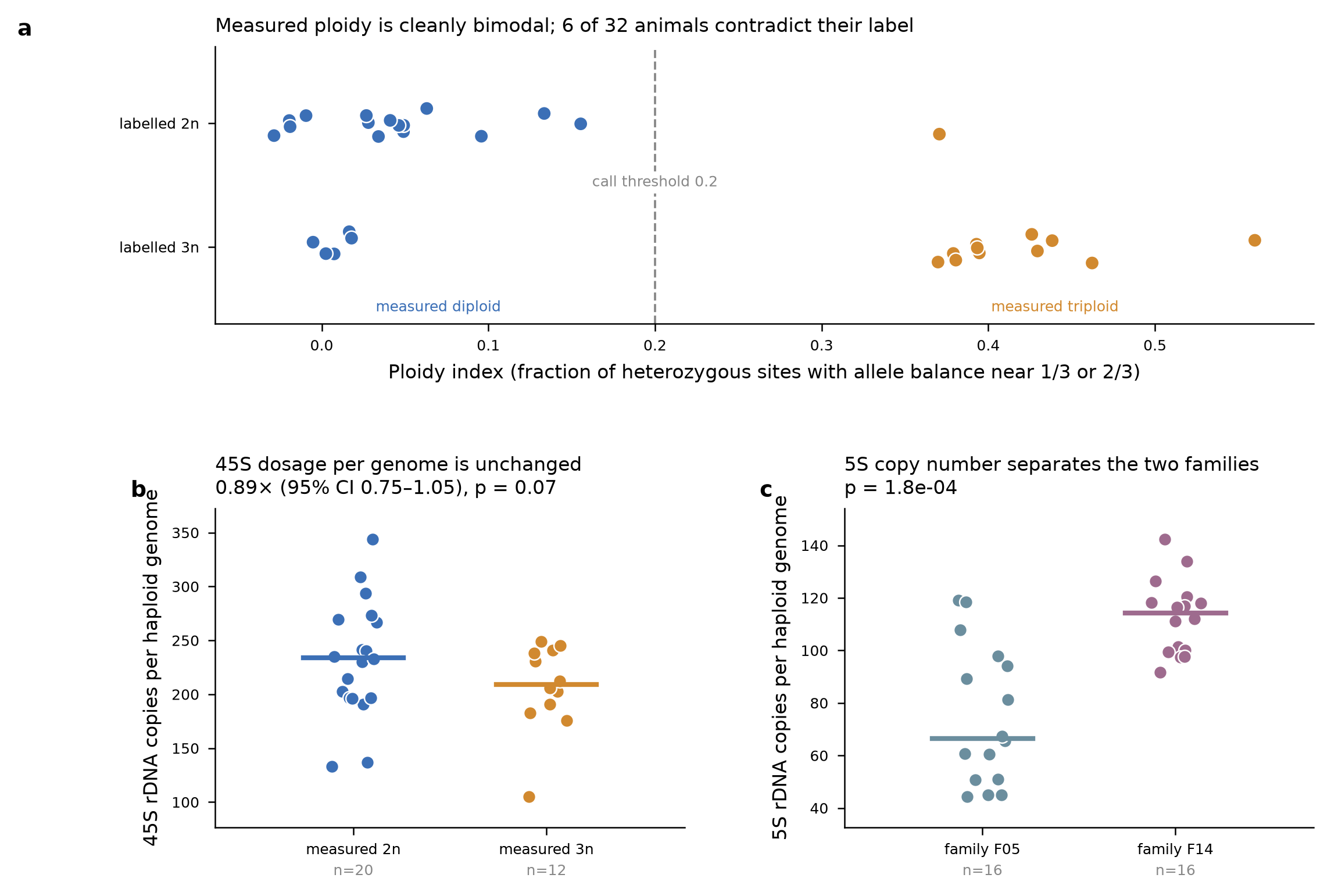
The ploidy index separated the animals cleanly into two groups (20 2n-like, 12 3n-like) with an empty separating band from 0.155 to 0.370 (Figure 2 a); the call threshold of 0.20 sits inside that gap, so the classification is insensitive to its exact value. Between 11,819 and 47,960 heterozygous sites per animal (median 38,789) entered the statistic.
Figure 1 shows why the calibration is necessary. At DP 6–12 a genuinely diploid animal produces prominent spikes at BAF 1/3 and 2/3 purely from depth discreteness — 2/6 and 4/6 are common binomial outcomes for a true 0.5 site — so the raw histogram cannot be read by eye (panel a). The simulated diploid reference reproduces those spikes, and the diagnostic signal is the relative depletion at 0.5 with mass displaced into the outer upper half, visible as the observation tracking the simulated-triploid outline instead (panel b). Every animal’s statistic falls within its own simulated 2n–3n range (panel e).
6 of 32 animals contradict their induction label:
| sample | family | label | measured | index | resampling 95% CI | het sites |
|---|---|---|---|---|---|---|
| F052n08 | F05 | 2n | 3n-like | 0.371 | 0.272 – 0.490 | 13,049 |
| F053n01 | F05 | 3n | 2n-like | 0.007 | -0.045 – 0.038 | 39,015 |
| F053n02 | F05 | 3n | 2n-like | -0.005 | -0.039 – 0.041 | 40,776 |
| F053n04 | F05 | 3n | 2n-like | 0.002 | -0.059 – 0.018 | 46,216 |
| F053n06 | F05 | 3n | 2n-like | 0.017 | -0.042 – 0.061 | 27,738 |
| F143n04 | F14 | 3n | 2n-like | 0.018 | -0.035 – 0.036 | 44,808 |
The discordance is asymmetric and dominated by induction failure: five labelled triploids read as diploid, four of them in family F05, whose indices sit essentially at the simulated diploid expectation (index <= 0.02) rather than at intermediate values. These are not marginal calls or mosaics — they are indistinguishable from diploids. One labelled diploid (F052n08) reads clearly triploid (index 0.37), consistent with a sample or label swap rather than with spontaneous triploidy.
Family F05 accounts for five of the six discordances, and its labelled-triploid group is effectively half diploid (4 of 8), whereas family F14 has 1 of 8. The nominal 2 x 2 design is therefore unbalanced in measured terms: F05 2n-like n = 11, F05 3n-like n = 5, F14 2n-like n = 9, F14 3n-like n = 7.
4.3 45S rDNA dosage per genome is unchanged by triploidy
Mean 45S copy number per haploid genome was 223 copies (range 105–344), and 5S 94 copies (44–142).
Triploidy did not detectably alter 45S dosage per haploid genome under either ploidy assignment (Figure 2 b). Full model output for both arms:
| arm | feature | ratio | 95% CI | p (ploidy) | p (family) | p (perm.) |
|---|---|---|---|---|---|---|
| pre-registered | 45S_transcribed_unit | 0.953 | 0.80 – 1.13 | 0.333 | 0.073 | 0.579 |
| pre-registered | 45S_18S | 0.941 | 0.79 – 1.12 | 0.259 | 0.055 | 0.475 |
| pre-registered | 45S_28S | 0.973 | 0.82 – 1.15 | 0.348 | 0.07 | 0.754 |
| pre-registered | 45S_5.8S | 0.963 | 0.81 – 1.14 | 0.338 | 0.087 | 0.661 |
| pre-registered | 5S_rRNA | 1.042 | 0.81 – 1.33 | 0.267 | 0.00029 | 0.664 |
| pre-registered | mitogenome | 0.781 | 0.62 – 0.99 | 0.560 | 0.55 | 0.057 |
| measured | 45S_transcribed_unit | 0.888 | 0.75 – 1.05 | 0.068 | 0.053 | 0.218 |
| measured | 45S_18S | 0.904 | 0.76 – 1.08 | 0.092 | 0.054 | 0.325 |
| measured | 45S_28S | 0.907 | 0.76 – 1.08 | 0.068 | 0.048 | 0.316 |
| measured | 45S_5.8S | 0.904 | 0.76 – 1.07 | 0.053 | 0.051 | 0.292 |
| measured | 5S_rRNA | 1.122 | 0.89 – 1.42 | 0.172 | 0.00018 | 0.553 |
| measured | mitogenome | 0.725 | 0.56 – 0.93 | 0.324 | 0.34 | 0.020 |
The pre-registered contrast gives 0.95-fold (95% CI 0.80–1.13, p = 0.33); the measured contrast gives 0.89-fold (95% CI 0.75–1.05, p = 0.068). The three transcribed subunits agree in magnitude and direction with the transcribed unit as a whole, as they must if the cassette is quantified consistently, and none reaches significance. The measured arm’s point estimate is a consistent 10% below unity across all 45S features with an interval that includes 1, which is a weak and internally consistent hint of slight per-genome reduction rather than a detected effect; with 20 versus 12 animals at the realised coverage, effects below roughly 25% are not resolvable here.
Because copy number is expressed per haploid genome, an unchanged per-genome value means copies per cell rise by half in triploids — the arrays are carried along by the extra genome complement rather than compensated.
4.4 Family, not ploidy, dominates 5S copy number
5S copy number did not track ploidy (1.12-fold, p = 0.17 measured) but differed sharply between families (p = 2e-04; Figure 2 c), with family means of 75 copies in F05 against 113 in F14 — a 1.5-fold difference, an order of magnitude larger than anything attributable to ploidy. The 45S features show the same pattern more weakly (p(family) between 0.000 and 0.054). Family background is the dominant axis of rDNA copy-number variation in this dataset.
4.5 Mitochondrial dosage corroborates the ploidy calls
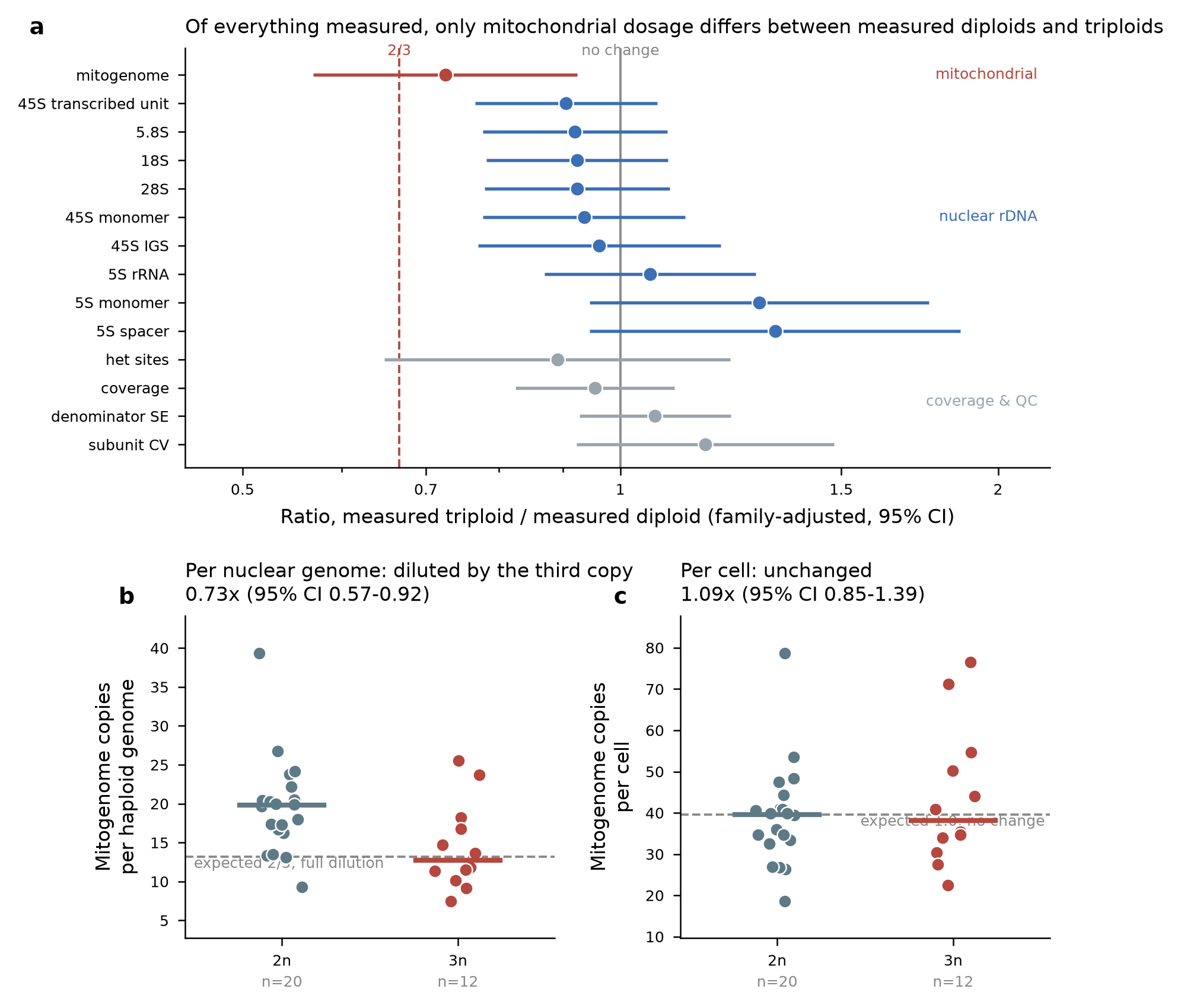
Mitogenome copy number per haploid nuclear genome is the only measured quantity besides the ploidy classifier itself that differs between measured diploids and measured triploids: 0.73-fold (95% CI 0.57–0.92, family-adjusted, p = 0.015) — 19.6 copies in diploids against 14.5 in triploids.
This is precisely what a ploidy-independent mitochondrial complement predicts. If a cell sets mitochondrial content without reference to nuclear ploidy, adding a third nuclear genome copy dilutes mitogenome copies per haploid nuclear genome by exactly 2/3 = 0.667. The observed ratio is distinguishable from no change (p = 0.015) and indistinguishable from full dilution. Re-expressed per cell — copy number times ploidy — the difference disappears: 1.09-fold (95% CI 0.84–1.40, p = 0.50), i.e. 39 against 43 mitogenomes per cell.
Two conclusions follow. Mitochondrial content per cell is unaffected by induced triploidy in these animals. And because mitochondrial read depth is an entirely separate signal from the allele balances used to call ploidy, its agreement with the 2/3 prediction is independent corroboration that the measured ploidy assignments are correct, including the six that contradict their labels.
A sweep of all non-classifier measured quantities against measured ploidy, each family-adjusted, is in data/ploidy_effect_sizes.csv and Figure 3: apart from the mitogenome, all nuclear rDNA features, coverage metrics and quality metrics are indistinguishable between measured diploids and measured triploids.
4.6 Exploratory: no gene-level dosage restructuring, but extensive family CNV
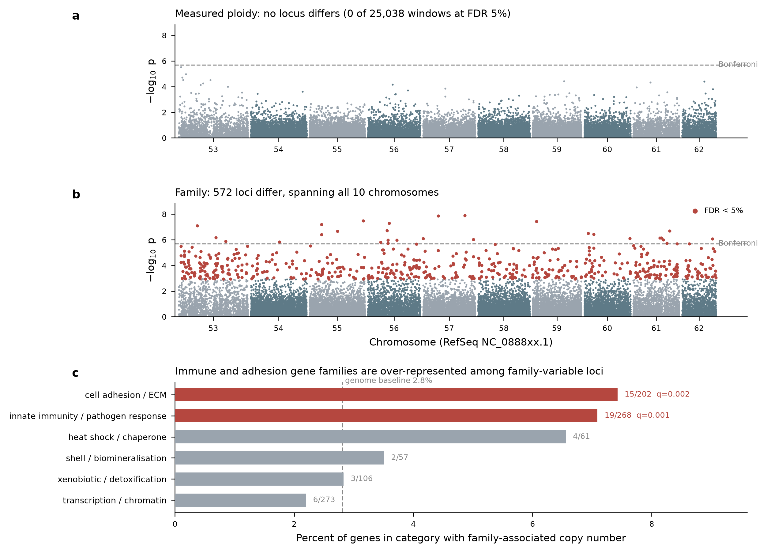
Across 25,038 1-kb windows — 17,526 of them inside 10,610 distinct protein-coding genes, roughly 41% of the annotated protein-coding gene set — no window was associated with ploidy at FDR 5% (minimum q = 0.076) or at Bonferroni (0 and 0 windows respectively; minimum p = 3e-06 against a 2e-06 threshold). Per-window effects are narrow: median absolute effect 1.15-fold, 99th percentile 2.04-fold (Figure 4 a).
This null must be read at the right scale. Per window, at the realised coverage and with 20 versus 12 animals, the minimum detectable effect at 80% power is 1.51-fold at alpha = 0.05 and 2.27-fold at the Bonferroni threshold, so individual genes varying with ploidy are not excluded. What is excluded is systematic restructuring: no locus stands out against the genome-wide background, and the genome-wide mean effect is +2.3% (95% CI +2.0% to +2.6%), a small residual global offset of the size expected from imperfect normalisation rather than a redistribution of dosage among genes. Triploidy scales the genome; it does not reorganise it — the same conclusion the pre-registered cassette analysis reached, extended to a large sample of protein-coding loci.
The same scan against family gives 572 windows at FDR 5% (2.3% of those tested), 29 surviving Bonferroni, distributed across all 10 chromosomes (Figure 4 b). Effects are large (median 2.2-fold, maximum 12.4-fold) and balanced in direction (314 higher in F14, 258 higher in F05). They are dispersed rather than clustered — only 26 of 572 lie within 5 kb of another hit — so these are scattered gene-level copy-number variants, not a few segmental duplications. 289 hit windows overlap a protein-coding gene, 295 distinct protein-coding genes in total.
Mappability does not explain them: both window sets were pre-selected for perfect mappability, so minimum mappability is 1.0 for every window in the scan, hits and non-hits alike, and GC content is indistinguishable between the two groups (Mann–Whitney p = 0.83).
Against a baseline of 2.8% of the 10,610 scanned protein-coding genes carrying a family-associated window, two categories are over-represented (Figure 4 c):
| category | genes with family-associated CN | rate | odds ratio | p | q |
|---|---|---|---|---|---|
| innate immunity / pathogen response | 19 / 268 | 7.1% | 2.78 | 0.000174 | 0.001 |
| cell adhesion / ECM | 15 / 202 | 7.4% | 2.90 | 0.000513 | 0.002 |
| heat shock / chaperone | 4 / 61 | 6.6% | 2.47 | 0.0893 | 0.179 |
| shell / biomineralisation | 2 / 57 | 3.5% | 1.27 | 0.473 | 0.683 |
| xenobiotic / detoxification | 3 / 106 | 2.8% | 1.02 | 0.569 | 0.683 |
| transcription / chromatin | 6 / 273 | 2.2% | 0.78 | 0.776 | 0.776 |
The immune hits include interferon-induced protein 44, an MDA5-type interferon-induced helicase, a cyclic GMP-AMP synthase-like receptor, tripartite motif proteins and perlucin-like lectins — gene families already reported as copy-number expanded in oysters.
5 Figures
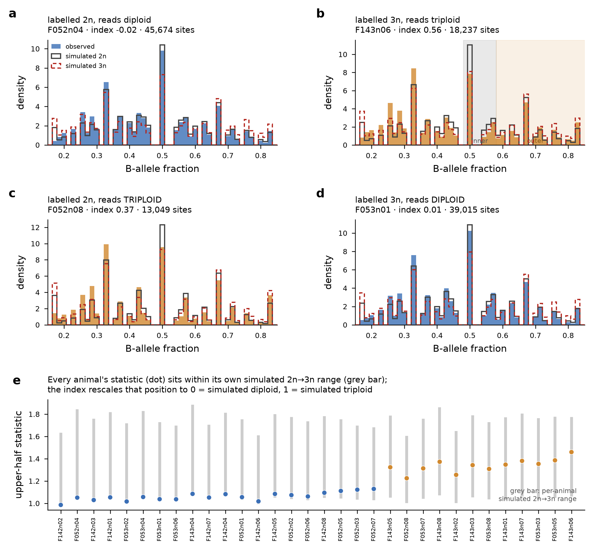
F052n08, labelled diploid, reading clearly triploid. (d) F053n01, labelled triploid, indistinguishable from a diploid. (e) Every animal’s observed upper-half statistic (dot, coloured by call) within its own simulated 2n→3n range (grey bar); the ploidy index rescales that position to 0 = simulated diploid, 1 = simulated triploid.
6 Discussion
Induced triploidy does not change rDNA dosage per genome. The pre-registered contrast is null, the measured contrast is null, and the three transcribed subunits agree. Copy number per haploid genome is a property of the arrays the animal inherited, and the extra genome complement in a triploid brings its arrays with it: copies per cell rise by half while copies per genome are unchanged. For ribosome biogenesis this is the simple expectation — triploid cells have 50% more rDNA and correspondingly more capacity — and nothing in these data suggests compensation at the array level.
The dominant axis is family, not ploidy. The 1.5-fold difference in 5S copy number between two families dwarfs any ploidy effect, and the exploratory scan makes the same point at genome scale: hundreds of loci separate the families, none separates the ploidies. Studies that treat rDNA copy number as a phenotype in this species will be dominated by family structure, and designs that do not block on family risk attributing to treatment what belongs to pedigree.
Ploidy labels require verification. Nearly one animal in five was mislabelled, and the failures were concentrated in one family, exactly the structure that would generate a spurious family-by-ploidy interaction had the labels been trusted. The verification here costs nothing extra — it reuses the same alignments as the copy-number analysis — and the mitochondrial dilution result provides an independent check on it from a signal with no shared machinery. We would argue that any sequencing-based study of induced polyploids should verify ploidy from the reads rather than from the treatment record. The concentration of failures in family F05 should be fed back to the induction programme; whether it reflects a treatment batch, a family-specific response, or a handling error cannot be resolved from these data.
What the nulls do and do not exclude. At the realised coverage the resolvable effect on 45S dosage is roughly 25%, and per-window gene-level effects below about 1.5-fold are not resolvable. These are not tight bounds. The claim supported here is the absence of a large or systematic effect, not the absence of any effect.
7 Limitations
- Coverage. Realised depth was 7.4x median against a 30x design target, because of 59% mean PCR duplication and low library complexity (18–27 million distinct fragments). All intervals are correspondingly wide. Deeper or less duplicated libraries would materially improve resolution; more reads from the same libraries would not, since complexity is the binding constraint.
- Design collapse. With 6 mislabelled animals, the balanced 2 x 2 design does not exist in measured terms, and measured ploidy is partly collinear with family. The measured contrast must be read as adjusted-for-family.
- Two families only. Family is the strongest effect in the data and is estimated from two families, so the magnitude of family variation is illustrated, not estimated.
- Arrays quantified by proxy. Copy number is depth over a single appended monomer relative to GC-matched single-copy windows. It measures total array content per genome, not array organisation, monomer heterogeneity or chromosomal distribution. The IGS estimate is flagged repeat-contaminated and is not interpreted.
- Gene-level scan reuses windows chosen for another purpose. Both window sets were selected to look single-copy and perfectly mappable, which is the least favourable place to find copy-number variation; the 572 family-associated loci are a floor, not an estimate. A 1-kb window inside a gene is not whole-gene copy number.
- Category assignment is keyword-based, not curated ontology enrichment, and 105 of the 295 family-associated genes have no functional description at all.
- Test statistics in the ploidy scan are mildly inflated (1,907 windows at p < 0.05 against 1,251 expected), consistent with residual depth structure not absorbed by the model. FDR control accounts for it, but the uncorrected p-value distribution should not be read as calibrated.
- Assumption diagnostics were not performed, and no cytometric or flow-based ploidy measurement was available to validate the sequence-based calls externally.
- Alignments were not retained, so BAM-level reanalysis requires realignment from FASTQ.
8 Tables
Table 1. Per-animal sequencing, coverage, duplication and ploidy metrics — data/sequencing_qc_summary.csv.
Table 2. Per-animal rDNA copy number, ploidy statistics and quality metrics — data/rdna_results_all32.csv.
Table 3. Model output for both analysis arms and all six pre-specified features — data/rdna_stats_results.csv (reproduced in full above).
Table 4. Family-associated copy-number loci and their gene assignments — data/family_cnv_genes.csv; category enrichment — data/family_cnv_enrichment.csv.
9 Data and code availability
Analysis code accompanying this report:
rdna_pipeline.sh— per-sample pipeline (trimming, alignment, depth, MAPQ check, variant calling), verbatim as executed; also at$D/code/.rdna_analysis.py— per-sample copy number and ploidy determination.rdna_stats.py— the two-arm statistical analysis.data/rdna_results_all32.csv— per-animal copy number, ploidy statistics and quality metrics.data/sequencing_qc_summary.csv— per-animal sequencing and coverage metrics.data/rdna_stats_results.csv— model output for both arms and all six pre-specified features.window_dosage_scan.csv.gz,data/family_cnv_genes.csv,data/family_cnv_enrichment.csv,gene_models.csv.gz— exploratory scan output.
Raw sequence data have not been deposited in a public archive at the time of writing; accessions must be added before publication.
Citations for the biological literature — oyster triploidy induction and performance, rDNA copy number variation, oyster immune gene family expansion — are not included here and must be added by the authors; this draft deliberately does not invent them.
10 Suggested citation
Roberts, S. B. 2026. Induced Triploidy Does Not Alter Per-Genome Ribosomal DNA Copy Number in the Pacific Oyster Magallana gigas. Current Findings. Available at: https://robertslab.github.io/current-findings/reports/oyster-triploidy-rdna-copy-number/
11 Version history
| Version | Date | Notes |
|---|---|---|
| 0.1 | 2026-08-31 | Migrated from rdna_manuscript_draft_figs.md |