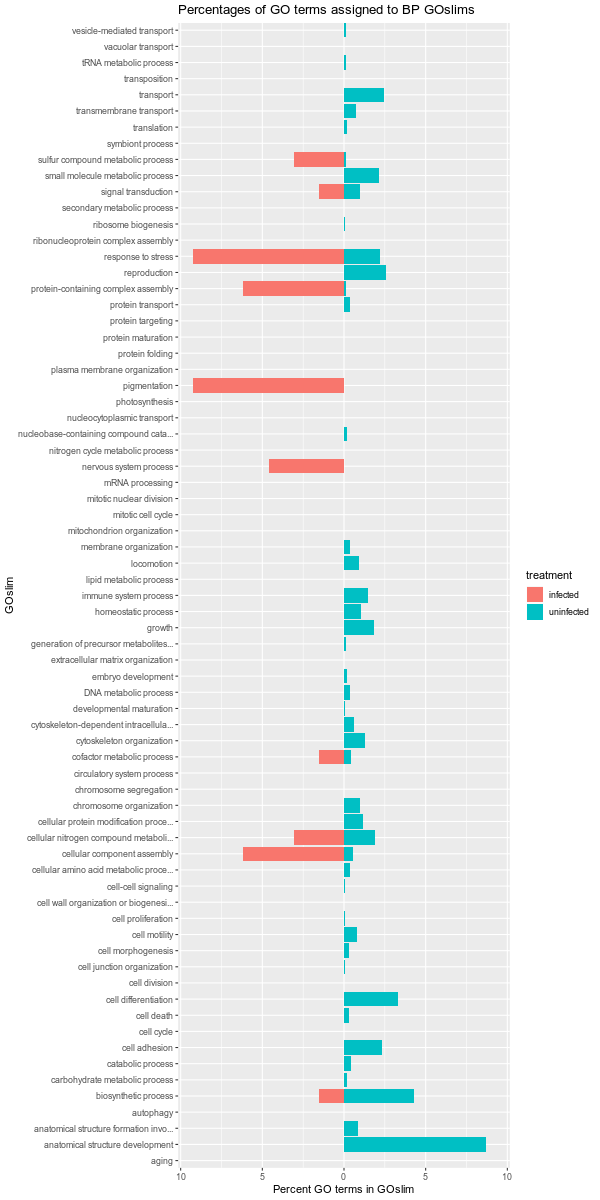
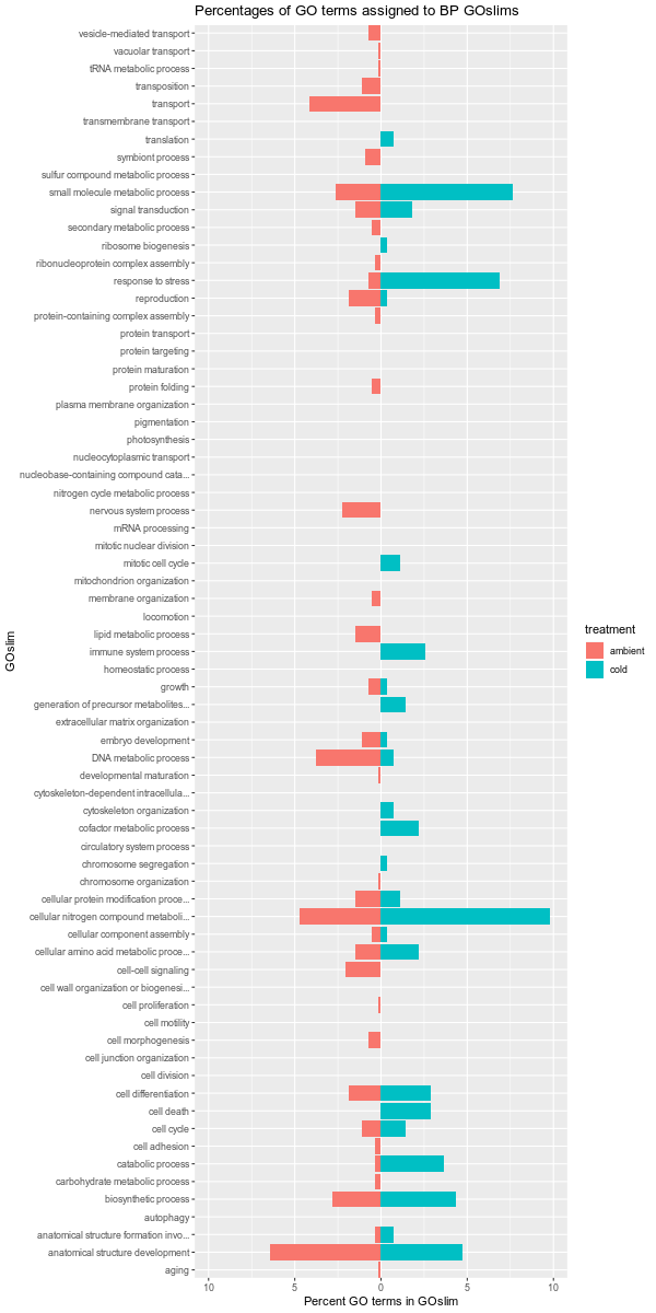
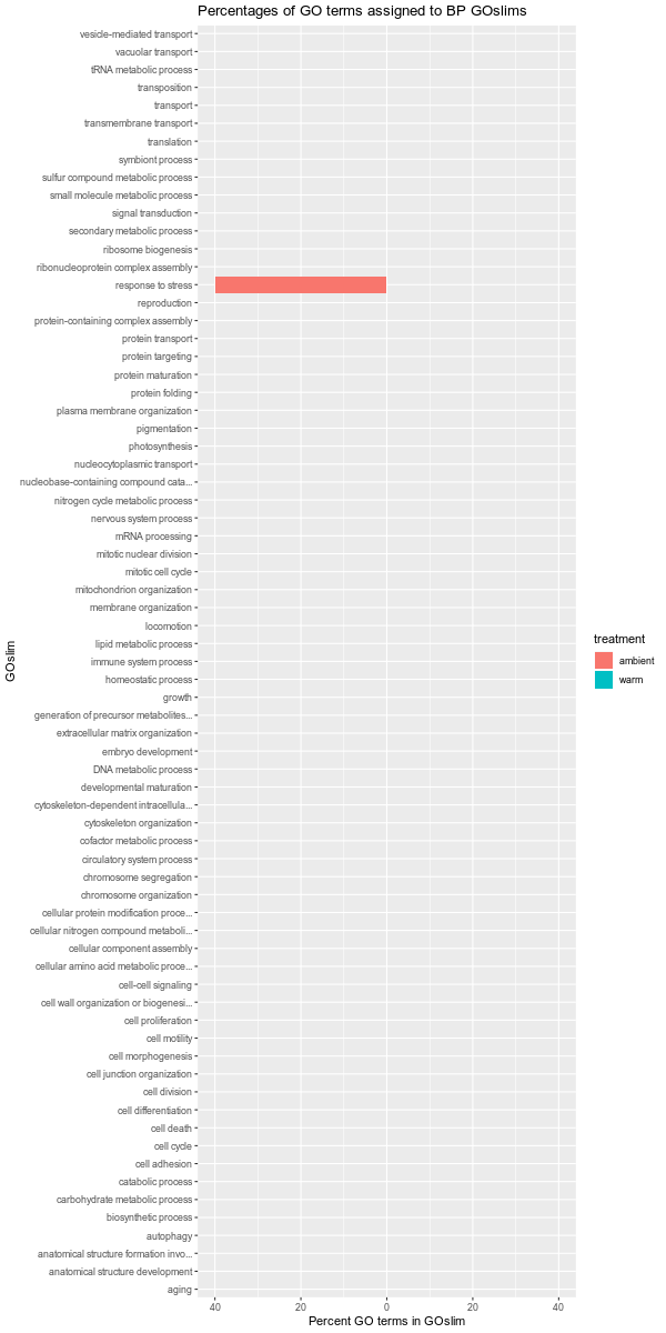
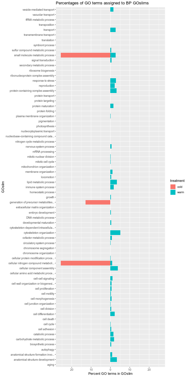
After running pairwise comparisons and identify differentially expressed genes (DEGs) on 20200422 and finding enriched gene ontology terms, I decided to map the GO terms to Biological Process GOslims. Additionally, I decided to try another level of comparison (I’m not sure how valid it is), whereby I will count the number of GO terms assigned to each GOslim and then calculate the percentage of GOterms that get assigned to each of the GOslim categories. The idea being that it might help identify Biological Processes that are “favored” in a given set of DEGs. I decided to set up “fancy” pyramid plots to view a given set of GO-GOslims for each DEG comparison.
All work was done in R. The initial counting/percentage calculations were done with the following R script (note: all of the followin R code are part of an R Project - link is in the RESULTS section of notebook). The R script uses a “flattened” set of the enriched GO terms identified by Trinity/GOseq, where flattened means one GO term per row. So, a gene may be represented multiple times, in multiple rows if there were multiple GO terms assigned to it by Trinity/GOseq.
The script then relies on the GSEABase package (Bioconductor) and the GO Consortium’s “Generic GO subset”:
After that, I plotted the outputs.
GO to GOslim R script:
library(GSEABase)
library(tidyverse)

#########################################################################
# Scipt to map C.bairdi DEG enriched GO terms to GOslims
# and identify the GO terms contributing to each GOslim
#########################################################################

### Download files and specify destination directory
download.file(url = "https://gannet.fish.washington.edu/Atumefaciens/20200422_cbai_DEG_basic_comparisons/D9-D12/edgeR.169728.dir/salmon.gene.counts.matrix.D12_vs_D9.edgeR.DE_results.P0.05_C1.D12-UP.subset.GOseq.enriched.flattened",
              destfile = "./data/D9-D12/salmon.gene.counts.matrix.D12_vs_D9.edgeR.DE_results.P0.05_C1.D12-UP.subset.GOseq.enriched.flattened")

download.file(url = "https://gannet.fish.washington.edu/Atumefaciens/20200422_cbai_DEG_basic_comparisons/D9-D12/edgeR.169728.dir/salmon.gene.counts.matrix.D12_vs_D9.edgeR.DE_results.P0.05_C1.D9-UP.subset.GOseq.enriched.flattened",
              destfile = "./data/D9-D12/salmon.gene.counts.matrix.D12_vs_D9.edgeR.DE_results.P0.05_C1.D9-UP.subset.GOseq.enriched.flattened")

download.file(url = "https://gannet.fish.washington.edu/Atumefaciens/20200422_cbai_DEG_basic_comparisons/D9-D26/edgeR.200352.dir/salmon.gene.counts.matrix.D26_vs_D9.edgeR.DE_results.P0.05_C1.D9-UP.subset.GOseq.enriched.flattened",
              destfile = "./data/D9-D26/salmon.gene.counts.matrix.D26_vs_D9.edgeR.DE_results.P0.05_C1.D9-UP.subset.GOseq.enriched.flattened")

download.file(url = "https://gannet.fish.washington.edu/Atumefaciens/20200422_cbai_DEG_basic_comparisons/D9-D26/edgeR.200352.dir/salmon.gene.counts.matrix.D26_vs_D9.edgeR.DE_results.P0.05_C1.D26-UP.subset.GOseq.enriched.flattened",
              destfile = "./data/D9-D26/salmon.gene.counts.matrix.D26_vs_D9.edgeR.DE_results.P0.05_C1.D26-UP.subset.GOseq.enriched.flattened")

download.file(url = "https://gannet.fish.washington.edu/Atumefaciens/20200422_cbai_DEG_basic_comparisons/D12-D26/edgeR.230922.dir/salmon.gene.counts.matrix.D12_vs_D26.edgeR.DE_results.P0.05_C1.D26-UP.subset.GOseq.enriched.flattened",
              destfile = "./data/D12-D26/salmon.gene.counts.matrix.D12_vs_D26.edgeR.DE_results.P0.05_C1.D26-UP.subset.GOseq.enriched.flattened")

download.file(url = "https://gannet.fish.washington.edu/Atumefaciens/20200422_cbai_DEG_basic_comparisons/ambient-cold/edgeR.267393.dir/salmon.gene.counts.matrix.ambient_vs_cold.edgeR.DE_results.P0.05_C1.ambient-UP.subset.GOseq.enriched.flattened",
              destfile = "./data/ambient-cold/salmon.gene.counts.matrix.ambient_vs_cold.edgeR.DE_results.P0.05_C1.ambient-UP.subset.GOseq.enriched.flattened")

download.file(url = "https://gannet.fish.washington.edu/Atumefaciens/20200422_cbai_DEG_basic_comparisons/ambient-cold/edgeR.267393.dir/salmon.gene.counts.matrix.ambient_vs_cold.edgeR.DE_results.P0.05_C1.cold-UP.subset.GOseq.enriched.flattened",
              destfile = "./data/ambient-cold/salmon.gene.counts.matrix.ambient_vs_cold.edgeR.DE_results.P0.05_C1.cold-UP.subset.GOseq.enriched.flattened")

download.file(url = "https://gannet.fish.washington.edu/Atumefaciens/20200422_cbai_DEG_basic_comparisons/ambient-warm/edgeR.297991.dir/salmon.gene.counts.matrix.ambient_vs_warm.edgeR.DE_results.P0.05_C1.warm-UP.subset.GOseq.enriched.flattened",
              destfile = "./data/ambient-warm/salmon.gene.counts.matrix.ambient_vs_warm.edgeR.DE_results.P0.05_C1.warm-UP.subset.GOseq.enriched.flattened")

download.file(url = "https://gannet.fish.washington.edu/Atumefaciens/20200422_cbai_DEG_basic_comparisons/ambient-warm/edgeR.297991.dir/salmon.gene.counts.matrix.ambient_vs_warm.edgeR.DE_results.P0.05_C1.ambient-UP.subset.GOseq.enriched.flattened",
              destfile = "./data/ambient-warm/salmon.gene.counts.matrix.ambient_vs_warm.edgeR.DE_results.P0.05_C1.ambient-UP.subset.GOseq.enriched.flattened")

download.file(url = "https://gannet.fish.washington.edu/Atumefaciens/20200422_cbai_DEG_basic_comparisons/cold-warm/edgeR.328585.dir/salmon.gene.counts.matrix.cold_vs_warm.edgeR.DE_results.P0.05_C1.warm-UP.subset.GOseq.enriched.flattened",
              destfile = "./data/cold-warm/salmon.gene.counts.matrix.cold_vs_warm.edgeR.DE_results.P0.05_C1.warm-UP.subset.GOseq.enriched.flattened")

download.file(url = "https://gannet.fish.washington.edu/Atumefaciens/20200422_cbai_DEG_basic_comparisons/cold-warm/edgeR.328585.dir/salmon.gene.counts.matrix.cold_vs_warm.edgeR.DE_results.P0.05_C1.cold-UP.subset.GOseq.enriched.flattened",
              destfile = "./data/cold-warm/salmon.gene.counts.matrix.cold_vs_warm.edgeR.DE_results.P0.05_C1.cold-UP.subset.GOseq.enriched.flattened")

download.file(url = "https://gannet.fish.washington.edu/Atumefaciens/20200422_cbai_DEG_basic_comparisons/infected-uninfected/edgeR.132470.dir/salmon.gene.counts.matrix.infected_vs_uninfected.edgeR.DE_results.P0.05_C1.infected-UP.subset.GOseq.enriched.flattened",
              destfile = "./data/infected-uninfected/salmon.gene.counts.matrix.infected_vs_uninfected.edgeR.DE_results.P0.05_C1.infected-UP.subset.GOseq.enriched.flattened")

download.file(url = "https://gannet.fish.washington.edu/Atumefaciens/20200422_cbai_DEG_basic_comparisons/infected-uninfected/edgeR.132470.dir/salmon.gene.counts.matrix.infected_vs_uninfected.edgeR.DE_results.P0.05_C1.uninfected-UP.subset.GOseq.enriched.flattened",
              destfile = "./data/infected-uninfected/salmon.gene.counts.matrix.infected_vs_uninfected.edgeR.DE_results.P0.05_C1.uninfected-UP.subset.GOseq.enriched.flattened")


### Set false discovery rate (FDR) filter, if desired
fdr <- as.character("1.0")

### Create list of files
goseq_files <- list.files(path = "./data",
                          pattern = "\\.GOseq.[de]",
                          recursive = TRUE,
                          full.names = TRUE)

### Set output filename suffix
output_suffix=("GOslims.csv")

### Strip path from goseq files
goseq_filename <- basename(goseq_files)

### Vector of GOslim ontologies (e.g. Biological Process = BP, Molecular Function = MF, Cellular Component = CC)
ontologies <- c("BP", "CC", "MF")

for (slim_ontology in ontologies) {

  ### Set GOOFFSPRING database, based on ontology group set above
  go_offspring <- paste("GO", slim_ontology, "OFFSPRING", sep = "")

  for (item in goseq_files) {

    ## Get max number of fields
    # Needed to handle reading in file with different number of columns in each row
    # as there may be multiple
    max_fields <- max(count.fields(item, sep = "\t"), na.rm = TRUE)

    ## Read in tab-delimited GOseq file
    # Use "max_fields" to populate all columns with a sequentially numbered header
    go_seqs <- read.delim(item,
                          col.names = paste0("V",seq_len(max_fields)))

    ## Filter enriched GOterms with false discovery rate
    goseqs_fdr <- filter(go_seqs, V8 <= as.numeric(fdr))

    ## Grab just the individual GO terms from the "category" column)
    goterms <- as.character(goseqs_fdr$V1)

    ### Use GSEA to map GO terms to GOslims

    ## Store goterms as GSEA object
    myCollection <- GOCollection(goterms)

    ## Use generic GOslim file to create a GOslim collection

    # I downloaded goslim_generic.obo from http://geneontology.org/docs/go-subset-guide
    # then i moved it to the R library for GSEABase in the extdata folder
    # in addition to using the command here - I think they're both required.
    slim <- getOBOCollection("./data/goslim_generic.obo")

    ## Map GO terms to GOslims and select Biological Processes group
    slimsdf <- goSlim(myCollection, slim, slim_ontology)

    ## Need to know the 'offspring' of each term in the ontology, and this is given by the data in:
    # GO.db::getFromNamespace(go_offspring, "GO.db")

    ## Create function to parse out GO terms assigned to each GOslim
    ## Courtesy Bioconductor Support: https://support.bioconductor.org/p/128407
    mappedIds <-
      function(df, collection, OFFSPRING)
      {
        map <- as.list(OFFSPRING[rownames(df)])
        mapped <- lapply(map, intersect, ids(collection))
        df[["go_terms"]] <- vapply(unname(mapped), paste, collapse = ";", character(1L))
        df
      }

    ## Run the function
    slimsdf <- mappedIds(slimsdf, myCollection, getFromNamespace(go_offspring, "GO.db"))

    ## Provide column name for first column
    slimsdf <- cbind(GOslim = rownames(slimsdf), slimsdf)
    rownames(slimsdf) <- NULL

    ### Prep output file naming structure

    ## Split filenames on periods
    ## Creates a list
    split_filename <- strsplit(item, ".", fixed = TRUE)

    ## Split filename on directories
    ## Creates a list
    split_dirs <- strsplit(item, "/", fixed = TRUE)

    ## Slice split_filename list from position 9 to the last position of the list
    ## Paste these together using a period
    goseq_filename_split <-paste(split_filename[[1]][9:lengths(split_filename)], collapse = ".")

    ## Slice split_dirs list at position

    ## Paste elements together to form output filename
    fdr_file_out <- paste("FDR", fdr, sep = "_")
    outfilename <- paste(goseq_filename_split, fdr_file_out, slim_ontology ,output_suffix, collapse = ".", sep = ".")

    ## Set output file destination and name
    ## Adds proper subdirectory from split_dirs list
    outfile_dest <- file.path("./analyses", split_dirs[[1]][3], outfilename)

    ## Write output file
    write.csv(slimsdf, file = outfile_dest, quote = FALSE, row.names = FALSE)


  }
}
Since I got “lazy” and didn’t want to try to figure out how to properly loop through all of the output files from the above script, I just made individual scripts to plot each set of comparison GO terms percentages assigned to GOslims. Here’s an example:
# Script to generate a "pyramid" plot
# comparing the percentages of enriched GO terms assinged
# to each category of Biological Process GOslims

library(dplyr)
library(ggplot2)


#####################################################
# Set the following variables for the appropriate comparisons/files
#####################################################
# Comparison
comparison <- "infected-uninfected"

# Treatments
treatment_01 <- "infected"
treatment_02 <- "uninfected"

# Read in first comparsion files
df1 <- read.csv("analyses/infected-uninfected/P0.05_C1.infected-UP.subset.GOseq.enriched.flattened.FDR_1.0.BP.GOslims.csv")

# Read in second comparison file
df2 <- read.csv("analyses/infected-uninfected/P0.05_C1.uninfected-UP.subset.GOseq.enriched.flattened.FDR_1.0.BP.GOslims.csv")


######################################################
# CHANGES BELOW HERE ARE PROBABLY NOT NECESSARY
######################################################

# GOslim categories
ontologies <- c("BP", "CC", "MF")

# Remove generic "biological_process" category
df1 <- df1[df1$GOslim != "GO:0008150",]
df2 <- df2[df2$GOslim != "GO:0008150",]

# Remove generic "cellular_component"  category
df1 <- df1[df1$GOslim != "GO:0005575",]
df2 <- df2[df2$GOslim != "GO:0005575",]


# Remove generic "molecular_function"  category
df1 <- df1[df1$GOslim != "GO:0003674",]
df2 <- df2[df2$GOslim != "GO:0003674",]

# Select columns
df1 <- df1 %>% select(Term, Percent)
df2 <- df2 %>% select(Term, Percent)

# Create treatment column and assign term to all rows
df1$treatment <- treatment_01
df2$treatment <- treatment_02

# Concatenate dataframes
df3 <- rbind(df1, df2)

# Filename for plot
pyramid <- paste(comparison, "GOslims", "BP", "png", sep = ".")
pyramid_path <- paste(comparison, pyramid, sep = "/")
pyramid_dest <- file.path("./analyses", pyramid_path)

# "Open" PNG file for saving subsequent plot
png(pyramid_dest, width = 600, height = 1200, units = "px", pointsize = 12)

# Create "pyramid" plot
ggplot(df3, aes(x = Term, fill = treatment,
                y = ifelse(test = treatment == treatment_01,
                           yes = -Percent,
                           no = Percent))) +
  geom_bar(stat = "identity") +
  scale_y_continuous(labels = abs, limits = max(df3$Percent) * c(-1,1)) +
  labs(title = "Percentages of GO terms assigned to BP GOslims", x = "GOslim", y = "Percent GO terms in GOslim") +
  scale_x_discrete(expand = c(-1,0)) +
  coord_flip()

# Close PNG file
dev.off()
RESULTS
Output folder (GitHub; R Project):
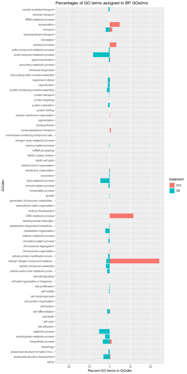
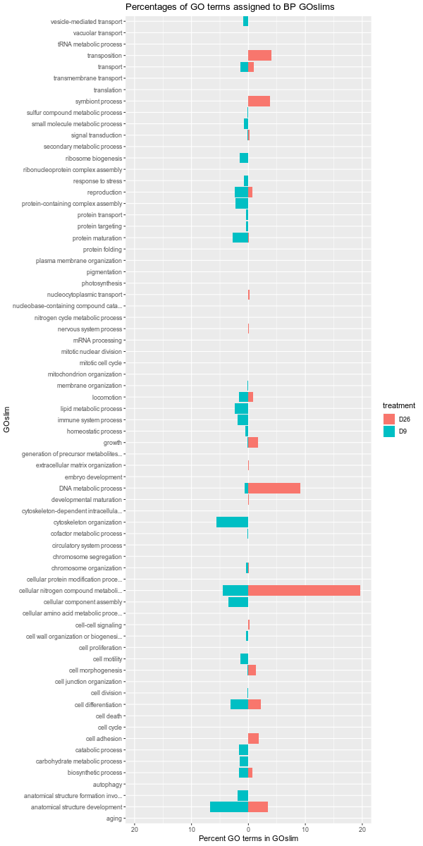
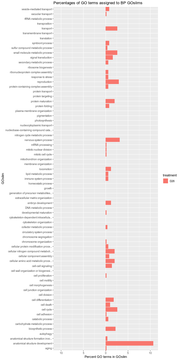
Images of each of the plots are below. Larger versions of the images can be viewed by clicking on the image. All images are 1200x600 pixels, so should be a reasonable size for viewing.
Also, it should be noted that the GOslim term “biological_process” was omitted from the plotting. This GOslim category is a “catchall” for any GO terms that do not fall into a GOslim category. As such, “biological_process” almost always makes up the bulk of the GOslim and this effectively compresses the plots, making it difficult to see any differences between the remaining GOslim categories. Knowing this explains why the percentages in each comparison never add up to 100%!
D9-D12
D9-D26
D12-D26
ambient-cold
ambient-warm
cold-warm
infected-uninfected
