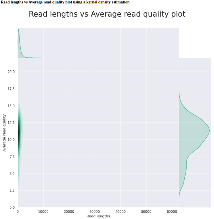
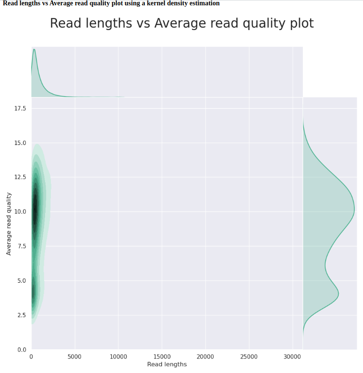
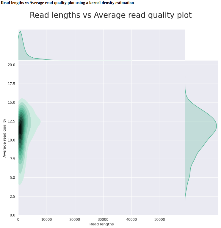
I previously converting our C.bairdi NanoPre sequencing data from the raw Fast5 format to FastQ format for our three sets of data:
Before proceeding with assembly and/or trying to tease out taxonomic differences (the C.bairdi-6129_403_26 is from an individual infected with Hematodinium), I want to get an idea of how the data looks. So, I’ve decided to process the sequencing_summary.txt file from each Fast5 conversion with NanoPlot. This software spits out some tables and some very nice visualizations to help get a better idea of how the sequencing runs look. This was run on Mox.
SBATCH script (GitHub):
#!/bin/bash
## Job Name
#SBATCH --job-name=cbai_nanoplot_nanopore-data
## Allocation Definition
#SBATCH --account=coenv
#SBATCH --partition=coenv
## Resources
## Nodes
#SBATCH --nodes=1
## Walltime (days-hours:minutes:seconds format)
#SBATCH --time=10-00:00:00
## Memory per node
#SBATCH --mem=120G
##turn on e-mail notification
#SBATCH --mail-type=ALL
#SBATCH --mail-user=samwhite@uw.edu
## Specify the working directory for this job
#SBATCH --chdir=/gscratch/scrubbed/samwhite/outputs/20200914_cbai_nanoplot_nanopore-data


###################################################################################
# These variables need to be set by user

# Load Anaconda
# Uknown why this is needed, but Anaconda will not run if this line is not included.
. "/gscratch/srlab/programs/anaconda3/etc/profile.d/conda.sh"


# Activate the NanoPlot Anaconda environment
conda activate nanoplot_env

# Set number of CPUs to use
threads=28

# Paths to reads
raw_reads_dir_array=(
"/gscratch/srlab/sam/data/C_bairdi/DNAseq/ont_FAL58500_04bb4d86_20102558-2729" \
"/gscratch/srlab/sam/data/C_bairdi/DNAseq/ont_FAL58500_94244ffd_20102558-2729" \
"/gscratch/srlab/sam/data/C_bairdi/DNAseq/ont_FAL86873_d8db260e_cbai_6129_403_26"
)

# Paths to programs
nanoplot=NanoPlot


###################################################################################


# Exit script if any command fails
set -e


# Capture this directory
wd=$(pwd)

# Inititalize array
programs_array=()


# Programs array
programs_array=("${nanoplot}")


# Loop through NanoPore data directories
# to run NanoPlot, FastQC, and MultiQC
for directory in "${!raw_reads_dir_array[@]}"
do


  # Capture NanoPore directory name
  dir_name=${raw_reads_dir_array[directory]##*/}

  # Make new directory and change to that directory
  mkdir "${dir_name}" && cd "$_"

  current_dir=$(pwd)


  # Run NanoPlot
  ## Sets readtype to 1D (default)
  ## Shows N50 on histograms
  ## Analysis perfomred using the sequencing summary file generated by
  ## guppy when converting from Fast5 to FastQ
  ${programs_array[nanoplot]} \
  --threads ${threads} \
  --outdir ${current_dir} \
  --readtype 1D \
  --N50 \
  --summary "${raw_reads_dir_array[directory]}"/sequencing_summary.txt

  # Change back to working directory
  cd "${wd}"

done


# Capture program options
for program in "${!programs_array[@]}"
do
    {
  echo "Program options for ${programs_array[program]}: "
    echo ""
    ${programs_array[program]} -h
    echo ""
    echo ""
    echo "----------------------------------------------"
    echo ""
    echo ""
} &>> program_options.log || true
done

# Document programs in PATH (primarily for program version ID)
{
date
echo ""
echo "System PATH for $SLURM_JOB_ID"
echo ""
printf "%0.s-" {1..10}
echo "${PATH}" | tr : \\n
} >> system_path.log
RESULTS
Very fast, 50s:

Output folder:
Each of the NanoPore NanoPlot analyses are in individual folders, linked below. Although I’ve only linked to the full report (in HTML format) for each, the plots and data present in the full report are also available in individual images/files within those folders.
C.bairdi-20102558-2729_Run-01 (FAL58500_94244ffd)
Output folder:
Full report (HTML):
| General summary | |
|---|---|
| Active channels | 491.0 |
| Mean read length | 821.6 |
| Mean read quality | 10.1 |
| Median read length | 533.0 |
| Median read quality | 10.6 |
| Number of reads | 78,720.0 |
| Read length N50 | 1,254.0 |
| Total bases | 64,672,912.0 |
Number, percentage and megabases of reads above quality cutoffs:
| Quality_cutoff | reads(count) | percentage | bases(count) |
|---|---|---|---|
| >Q5 | 73315 | (93.1%) | 60.5Mb |
| >Q7 | 67186 | (85.3%) | 56.5Mb |
| >Q10 | 46724 | (59.4%) | 41.4Mb |
| >Q12 | 20961 | (26.6%) | 20.6Mb |
| >Q15 | 966 | (1.2%) | 0.8Mb |
Top 5 highest mean basecall quality scores and their read lengths:
| Rank | mean_quality | read_length(bp) | bases(count) |
|---|---|---|---|
| 1 | 22 | (682) | 60.5Mb |
| 2 | 19.8 | (471) | 56.5Mb |
| 3 | 19.1 | (414) | 41.4Mb |
| 4 | 19.1 | (1539) | 20.6Mb |
| 5 | 19 | (234) | 0.8Mb |
Top 5 longest reads and their mean basecall quality score:
| Rank | read_length(bp) | mean_quality_score |
|---|---|---|
| 1 | 62629 | (3.3) |
| 2 | 51173 | (3.5) |
| 3 | 45909 | (3.0) |
| 4 | 44689 | (3.4) |
| 5 | 42633 | (3.0) |

C.bairdi-20102558-2729_Run-02 (FAL58500_04bb4d86)
Output folder:
Full report (HTML):
| GENERAL SUMMARY | |
|---|---|
| Active channels | 424.0 |
| Mean read length | 845.5 |
| Mean read quality | 8.7 |
| Median read length | 521.0 |
| Median read quality | 9.3 |
| Number of reads | 21,519.0 |
| Read length N50 | 1,406.0 |
| Total bases | 18,195,027.0 |
Number, percentage and megabases of reads above quality cutoffs:
| Quality_cutoff | reads(count) | percentage | bases(count) |
|---|---|---|---|
| >Q5 | 17207 | (80.0%) | 15.4Mb |
| >Q7 | 14864 | (69.1%) | 13.9Mb |
| >Q10 | 8797 | (40.9%) | 8.9Mb |
| >Q12 | 3257 | (15.1%) | 3.6Mb |
| >Q15 | 121 | (0.6%) | 0.1Mb |
Top 5 highest mean basecall quality scores and their read lengths:
| Rank | mean_quality | read_length(bp) |
|---|---|---|
| 1 | 18.3 | (323) |
| 2 | 17.8 | (1064) |
| 3 | 17.4 | (201) |
| 4 | 17.3 | (761) |
| 5 | 16.9 | (642) |
Top 5 longest reads and their mean basecall quality score:
| Rank | read_length(bp) | mean_quality_score |
|---|---|---|
| 1 | 31170 | (3.4) |
| 2 | 28158 | (3.2) |
| 3 | 27016 | (3.3) |
| 4 | 24304 | (3.6) |
| 5 | 15552 | (2.9) |

C.bairdi-6129_403_26 (FAL86873_d8db260e)
Output folder:
Full report (HTML):
| GENERAL SUMMARY | |
|---|---|
| Active channels | 503 |
| Mean read length | 2254.5 |
| Mean read quality | 10.9 |
| Median read length | 965 |
| Median read quality | 11.2 |
| Number of reads | 506495 |
| Read length N50 | 5232 |
| Total bases | 1141890358 |
Number, percentage and megabases of reads above quality cutoffs:
| Quality_cutoff | reads(count) | percentage | bases(count) |
|---|---|---|---|
| >Q5 | 493598 | (97.5%) | 1124.9Mb |
| >Q7 | 465033 | (91.8%) | 1075.5Mb |
| >Q10 | 343296 | (67.8%) | 880.9Mb |
| >Q12 | 186709 | (36.9%) | 568.7Mb |
| >Q15 | 7394 | (1.5%) | 17.9Mb |
Top 5 highest mean basecall quality scores and their read lengths:
| Rank | mean_quality | read_length(bp) |
|---|---|---|
| 1 | 20.6 | (980) |
| 2 | 20.2 | (1228) |
| 3 | 19.7 | (902) |
| 4 | 19.6 | (466) |
| 5 | 19.6 | (757) |
Top 5 longest reads and their mean basecall quality score:
| Rank | read_length(bp) | mean_quality_score |
|---|---|---|
| 1 | 58854 | (11.8) |
| 2 | 57315 | (10.8) |
| 3 | 51351 | (11.5) |
| 4 | 51326 | (13.7) |
| 5 | 49825 | (12.9) |

First, we should compare the two C.bairdi-20102558-2729 runs (degraded input DNA, no Hematodinium infection), as these were the same sample, run on the same flowcell.
Basically, the second run on the flowcell performs worse in every metric: fewer reads, lower quality scores, shorter read lengths, etc. This is despite the fact that this flowcell was run for nearly 4.5x longer period of time (72hrs vs. 16hrs). This isn’t terribly surprising, as the second run started with only 414 available pores, which is well below the ONT-suggested minimum of 800 pores for a “good” flowcell, but it is interesting to see the actual impacts on sequencing that this has.
The C.bairdi-6129_403_26 run (high quality input DNA, with Hematodinium infection) is a better example of what to expect when using non-degraded DNA. Every metric is substantially better than the C.bairdi-20102558-2729 runs.
Now, how to proceed? First, I think I’ll just get an assembly made, utilizing all three sets of data, despite the presence of Hematodinium in the C.bairdi-6129_403_26 run. I’ll tackle the assembly using Flye, as it seems straightforward, is specifically designed for long read assembly, and has built-in assembly “polishing”. This will be a start.
In regards to teasing out Hematodinium sequences, I’ll probably go through the DIAMOND BLASTx -> MEGAN6 process that I’ve used throughout our C.baird RNAseq project for transcriptome assemblies. MEGAN6 can handle long reads and makes taxonomic read extraction straightforward.