INTRO
This notebook performs pair-wise comparisons of qPCR gene expression, normalized to GAPDH expression. It calculates delta Cq, delta delta Cq, and fold changes in expression. Additionally, it generates box plots (delta Cq), and bar plots (fold change expression).
I’ve provided a summary of the various pair-wise comparisons immediately below, but you might want to just skip to the plots, as the summary and the notebook content is very lengthy.
SUMMARY
t-tests (Delta Cq)
Seed vs. Adult
These genes had p-values <= 0.05:
- VIPERIN
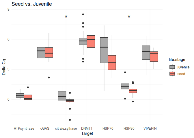
Seed vs. Juvenile
These genes had p-values <= 0.05:
citrate synthase
HSP90
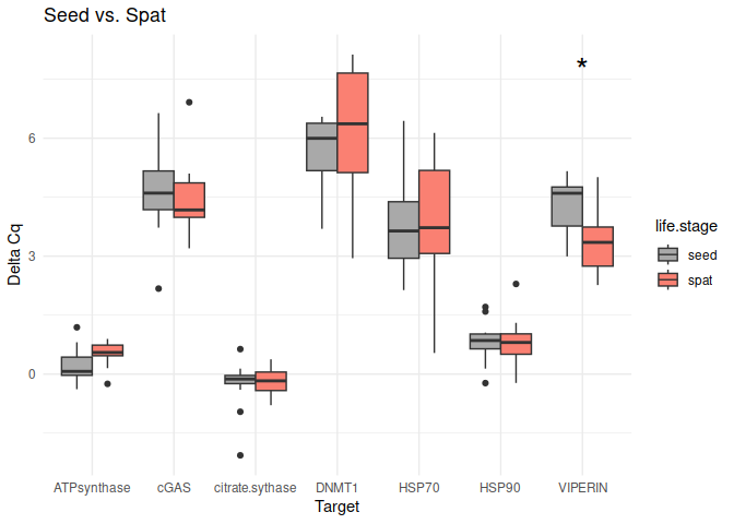
Seed vs. Spat
These genes had p-values <= 0.05:
- VIPERIN
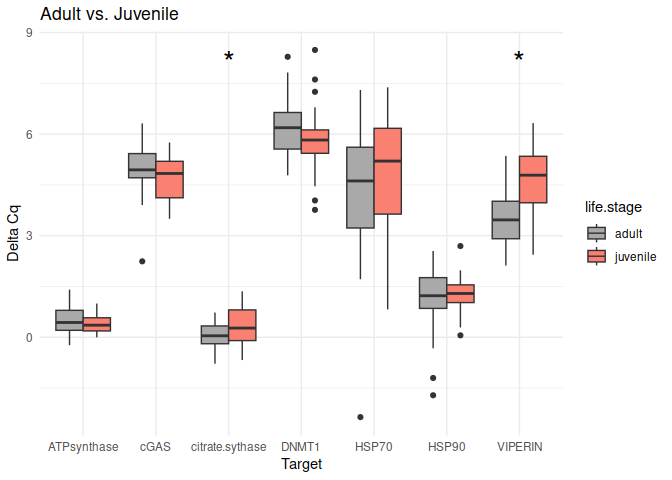
Adult vs. Juvenile
The genes had p-values <= 0.05:
citrate synthase
VIPERIN
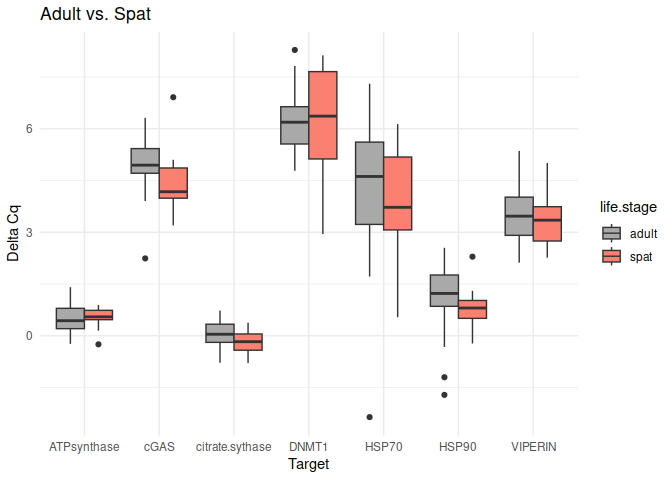
Adult vs. Spat
No genes had p-values <= 0.05
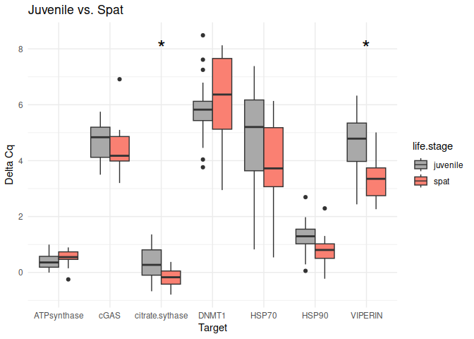
Juvenile vs. Spat
The genes had p-values <= 0.05:
citrate synthase
VIPERIN
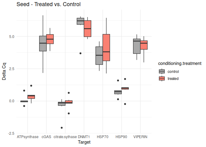
Seed - Conditioning Treated vs. Control
No genes had p-values <= 0.05
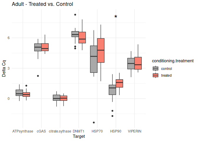
Adult - Conditioning Treated vs. Control
The genes had p-values <= 0.05:
- HSP90
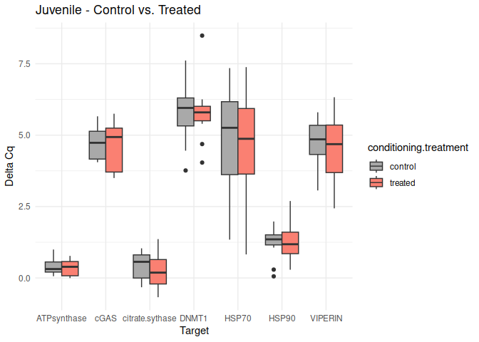
Juvenile - Conditioning Treated vs. Control
No genes had p-values <= 0.05
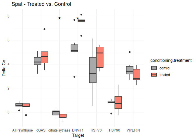
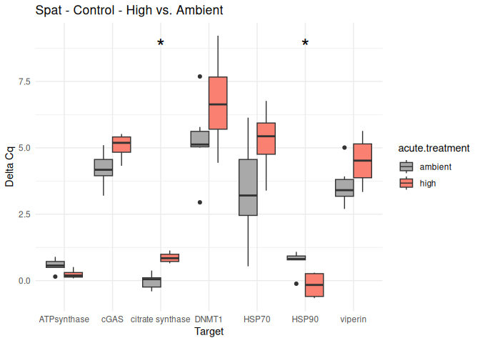
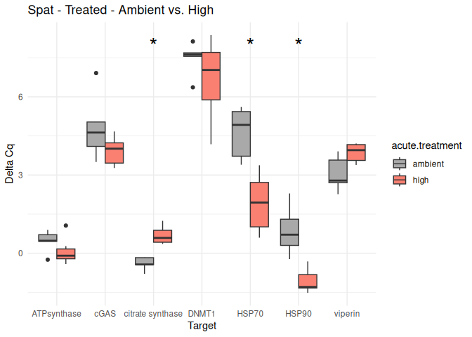
Spat - Conditioning Treated vs. Control
The genes had p-values <= 0.05:
citrate synthase
DNMT1
Adult - Acute Ambient vs. High
No genes had p-values <= 0.05
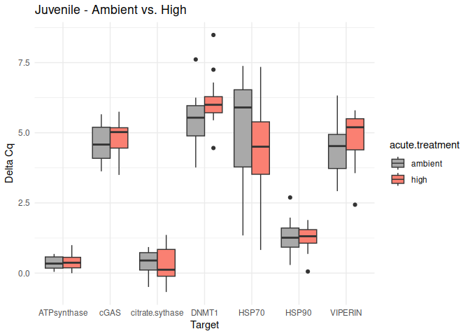
Juvenile - Acute Ambient vs. High
No genes had p-values <= 0.05
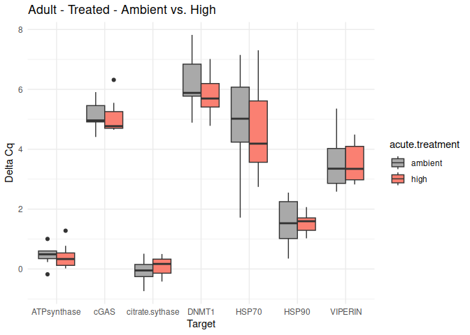
Adult - Conditioning Treated: Acute Ambient vs. High
No genes had p-values <= 0.05
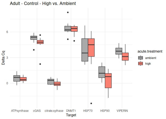
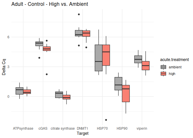
Adult - Conditioning Control: Acute Ambient vs. High
No genes had p-values <= 0.05
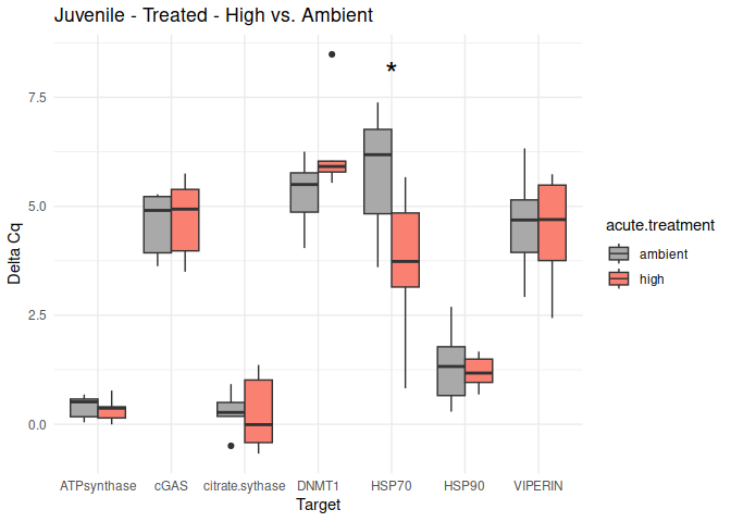
Juvenile - Conditioning Treated: Acute Ambient vs. High
The genes had p-values <= 0.05:
- HSP70
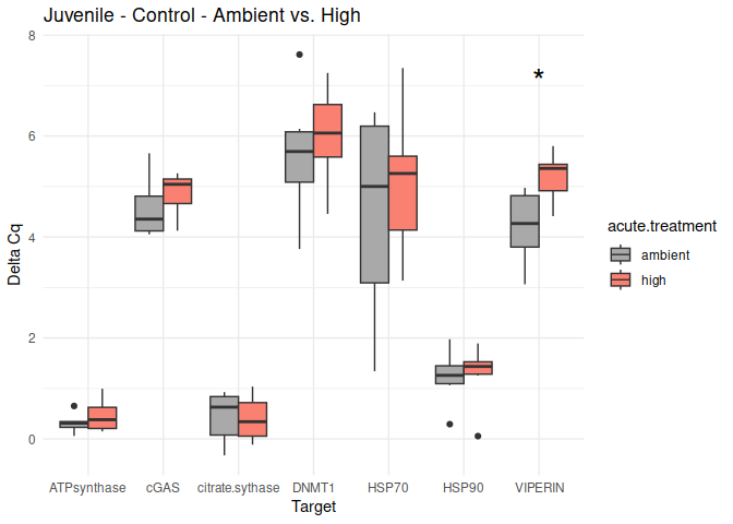
Juvenile - Conditioning Control: Acute Ambient vs. High
The genes had p-values <= 0.05:
- VIPERIN
Gene Expression (delta delta Cq or fold change)
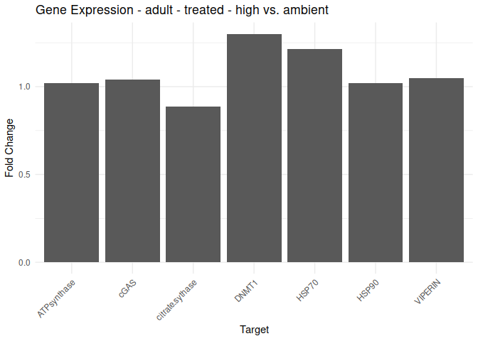
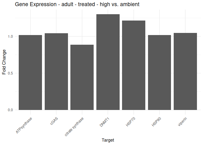
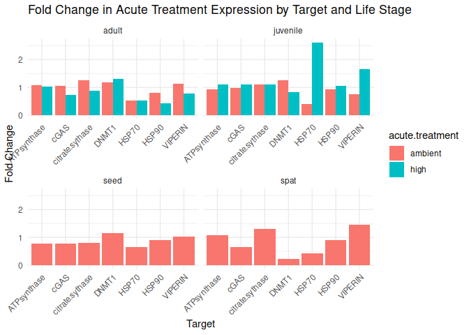
Adult - Conditioning Treated: Acute High vs. Ambient
All genes show elevated expression relative to Ambient.
Fold change is at similar levels across all genes, with DNMT1 and HSP70 being the highest.
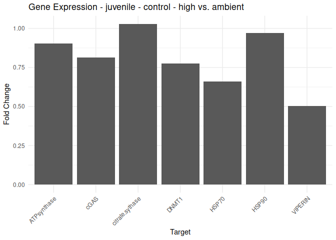
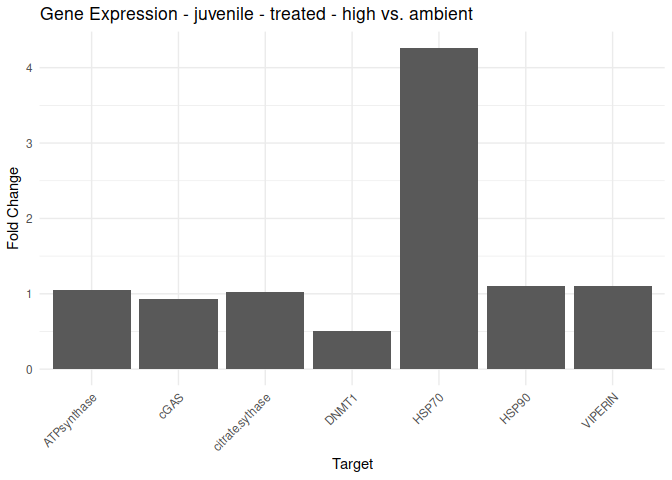
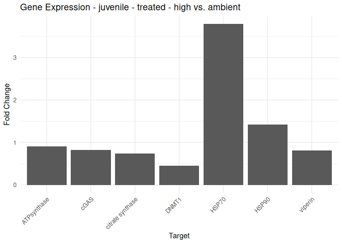
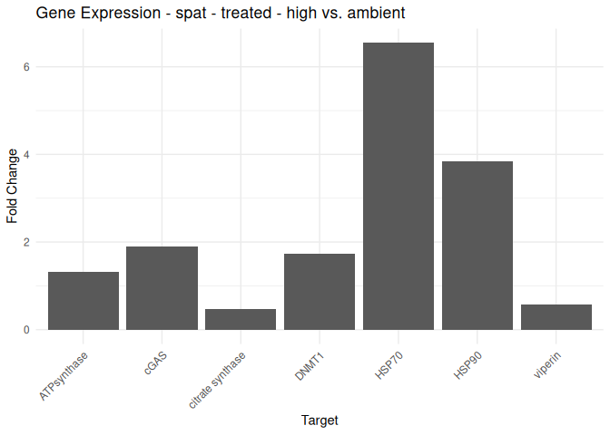
Juvenile - Conditioning Treated: Acute High vs. Ambient
All genes show elevated expression relative to Ambient.
HSP70 shows ~4-fold higher fold change in expression compared to most of the other genes.
DNMT1 exhibits fold change expression ~1/2 that of most of the other genes.
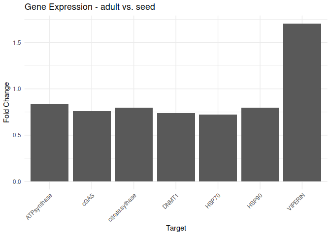
Adult - Adult vs. Seed
All genes show elevated expression relative to Seed.
VIPERIN exhibits fold change in expression >2-fold higher than the other genes.
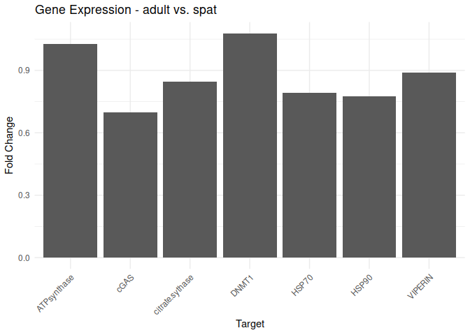
Adult - Adult vs. Spat
All genes show elevated expression relative to Spat.
All genes have similar fold changes in expression, with ATP synthase and DNMT1 showing the highest levels of fold change in expression.
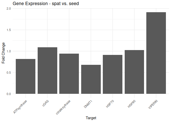
Adult - Spat vs. Seed
All genes show elevated expression relative to Seed.
Most genes have similar fold changes in expression.
VIPERIN exhibits fold change in a expression ~2-fold higher than the other genes.
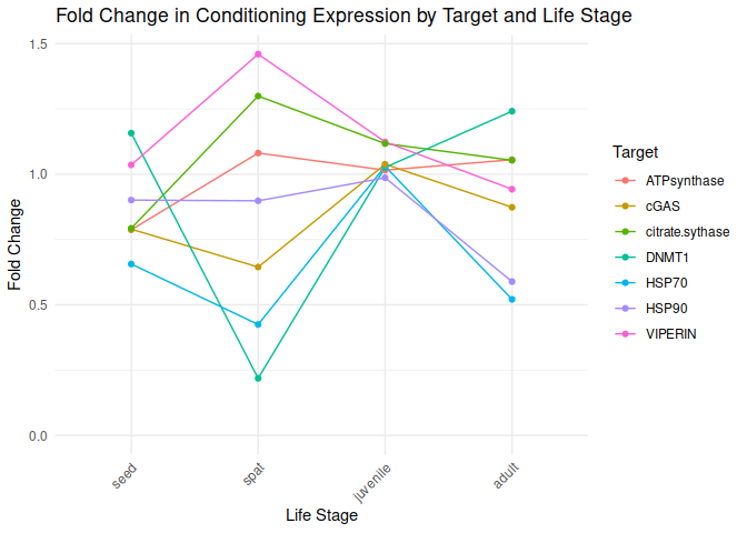
Conditioning by Target and Lifestage
All genes show elevated expression relative to Control.
VIPERIN, citrate synthase, and ATP synthase show an initial increase in fold change expression from seed to spat life stages, declining to juvenile and adult lifestages.
HSP90 shows level fold changes in expression across seed, spat, and juvenile lifestages, followed by a decrease in the adult stage.
DNMT1 exhibits a drastic decrease in fold change expression from seed to spat, followed by a substantial increase from spat to adult.
cGAS and HSP70 exhibit decreases from seed to spat, followed by a sharp increase from spat to juvenile. This is followed by a moderate decrease from juvenile to adult by cGAS and a sharp decrease in HSP70.
The post below is markdown generated from 01.01-qPCR.Rmd (commit 71b99c4).
Ariana added everything after ### 9.2.5 Acute treatment comparison.
1 Description
This notebook performs pair-wise comparisons of qPCR gene expression, normalized to GAPDH expression. It calculates delta Cq, delta delta Cq, and fold changes in expression. Additionally, it generates box plots (delta Cq), and bar plots (fold change expression).
2 Set variables
2.1 Set sample groups
Groups are named in the following fashion:
<life.stage>.<conditioning.treatment>.<acute.treatment>
This allows for parsing downstream.
NOTE: Below is the full set of groups for the entire experiment. For the current qPCR analysis, seed and spat do not have acute treatments; just conditioning treatments.
seed.control.ambient=c("29", "40", "55", "63", "69", "101", "119", "122", "155", "164", "187", "202", "209", "214", "233", "236", "275")
seed.control.high=c("42", "59", "60", "62", "86", "102", "140", "176", "177", "184", "192", "223", "234", "243", "244", "254", "264")
seed.treated.ambient=c("14", "48", "66", "72", "89", "115", "129", "138", "156", "182", "191", "201", "227", "239", "270", "277", "280")
seed.treated.high=c("15", "19", "24", "88", "92", "105", "111", "113", "120", "128", "161", "200", "211", "256", "257", "266", "285")
spat.control.ambient=c("11", "30", "36", "52", "77", "114", "134", "142", "144", "183", "193", "229", "230", "231", "240", "272", "287")
spat.control.high=c("27", "74", "93", "96", "97", "137", "143", "153", "168", "178", "189", "206", "262", "274", "282", "284", "289")
spat.treated.ambient=c("9", "13", "38", "46", "47", "121", "145", "151", "174", "194", "197", "198", "216", "235", "241", "252", "291")
spat.treated.high=c("6", "25", "50", "78", "124", "126", "131", "160", "163", "172", "220", "226", "242", "253", "296", "298")
juvenile.control.ambient=c("18", "57", "65", "75", "79", "104", "110", "123", "125", "171", "175", "205", "238", "273", "279", "293", "317")
juvenile.control.high=c("12", "39", "43", "49", "71", "130", "141", "146", "150", "170", "195", "297", "301", "324", "351", "355", "371")
juvenile.treated.ambient=c("1", "34", "64", "83", "98", "147", "152", "158", "162", "169", "188", "271", "295", "310", "357", "361", "381")
juvenile.treated.high=c("28", "53", "61", "73", "81", "106", "109", "139", "149", "173", "181", "213", "290", "302", "311", "364", "392")
adult.control.ambient=c("3", "5", "13*", "16", "17", "80", "87", "94", "148", "159", "179", "180", "250", "258", "268", "312", "326", "330", "334", "346", "360", "377", "379", "386")
adult.control.high=c("20", "23", "26", "32", "33", "67", "70", "90", "107", "132", "135", "157", "166", "186", "207", "215", "248", "316", "341", "344", "349", "382", "394", "395")
adult.treated.ambient=c("7", "31", "35", "37", "41", "54", "84", "100", "112", "116", "118", "133", "154", "199", "203", "204", "208", "219", "294", "318", "339", "353", "363", "378")
adult.treated.high=c("21", "22", "45", "82", "85", "91", "95", "99", "103", "108", "117", "127", "165", "185", "190", "196", "232", "237", "245", "263", "276", "306", "343", "374")
2.2 Assign groups to list
# Combine vectors into lists
# Used for adding treatment info and/or subsetting downstream

groups_list <- list(juvenile.control.ambient = juvenile.control.ambient,
                                   juvenile.control.high = juvenile.control.high,
                                   juvenile.treated.ambient = juvenile.treated.ambient,
                                   juvenile.treated.high = juvenile.treated.high,
                                   adult.control.ambient = adult.control.ambient,
                                   adult.control.high = adult.control.high,
                                   adult.treated.ambient = adult.treated.ambient,
                                   adult.treated.high = adult.treated.high,
                                   seed.control.ambient = seed.control.ambient,
                                   seed.control.high = seed.control.high,
                                   seed.treated.ambient = seed.treated.ambient,
                                   seed.treated.high = seed.treated.high,
                                   spat.control.ambient = spat.control.ambient,
                                   spat.control.high = spat.control.high,
                                   spat.treated.ambient = spat.treated.ambient,
                                   spat.treated.high = spat.treated.high)
3 Functions
3.1 Calculate delta Cq
Normalized to designated normalizing gene
calculate_delta_Cq <- function(df) {
  df <- df %>%
    group_by(Sample) %>%
    mutate(delta_Cq = Cq.Mean - Cq.Mean[Target == "GAPDH"]) %>%
    ungroup()

  return(df)
}
3.2 Create delta Cq boxplots
3.2.1 Lifestage comparison
# Function to create box plots for each comparison
create_boxplot_delta_Cq <- function(data, comparison, t_test_results) {
  # Extract life stages from comparison
  life_stages <- unlist(strsplit(comparison, "\\."))

  # Debugging: Print life stages
  # print(paste("Life stages for comparison:", comparison))
  # print(life_stages)

  # Filter data for the relevant life stages
  filtered_data <- data %>%
    filter(life.stage %in% life_stages)

  # Debugging: Print filtered data
  # print("Filtered data:")
  # print(filtered_data)

  # Check if both life stages are included
  if (!all(life_stages %in% unique(filtered_data$life.stage))) {
    stop("Not all life stages are included in the filtered data")
  }

  y_limits <- range(filtered_data$delta_Cq, na.rm = TRUE)

  # Debugging: Print y_limits
  # print("Y limits:")
  # print(y_limits)

  # Filter t_test_results for the current comparison
  t_test_results_filtered <- t_test_results %>%
    filter(comparison == !!comparison)

  # Debugging: Print filtered t_test_results
  # print("Filtered t_test_results:")
  # print(t_test_results_filtered)

  # Filter t_test_results for asterisks
  t_test_results_with_asterisks <- t_test_results_filtered %>%
    filter(asterisk != "")

  # Debugging: Print t_test_results_with_asterisks
  # print("t_test_results_with_asterisks:")
  # print(t_test_results_with_asterisks)

  formatted_title <- paste0(toupper(substring(life_stages[1], 1, 1)), substring(life_stages[1], 2),
                            " vs. ",
                            toupper(substring(life_stages[2], 1, 1)), substring(life_stages[2], 2))

  boxplot <- ggplot(filtered_data, aes(x = Target, y = delta_Cq, fill = life.stage)) +
    geom_boxplot(position = position_dodge(width = 0.75)) +
    theme_minimal() +
    theme(legend.position = "right") +
    scale_fill_manual(values=c("darkgray", "salmon", "lightblue", "lightgreen")) +
    ylim(y_limits) +
    labs(x = "Target", y = "Delta Cq", title = formatted_title) +
    # Highlighted section: Adds asterisks
    geom_text(data = t_test_results_with_asterisks,
              aes(x = Target, y = y_limits[2] - 1, label = asterisk),
              vjust = -0.5, size = 8, color = "black", inherit.aes = FALSE)

  print(boxplot)
}
3.2.2 Conditioning comparisons
- Extract Life Stage and Conditioning Treatments:
- The comparison string is split into its components (
life_stage,treatment1, andtreatment2).
- Filter Data:
- The filtered_data data frame is filtered to include only the rows with the relevant life stage and conditioning treatments.
- Check for Both Treatments:
- Ensure that both treatments are included in the
filtered_data.
- Filter T-Test Results:
The
t_test_results_filtereddata frame is filtered for the specific comparison.The
t_test_results_with_asterisksdata frame is created to include only the rows with asterisks.
- Format the Title:
The
formatted_titlevariable is created by capitalizing the first letter of each component and concatenating them with ” - ” and ” vs. ” in between.This should create box plots comparing conditioning treatments within each life stage, with titles formatted as
<life.stage> - Treated vs. Control.
# Function to create box plots for each comparison of conditioning treatments within life stages
create_boxplot_conditioning <- function(data, comparison, t_test_results) {
  # Extract life stage and conditioning treatments from comparison
  comparison_parts <- unlist(strsplit(comparison, "\\."))
  life_stage <- comparison_parts[1]
  treatment1 <- comparison_parts[2]
  treatment2 <- comparison_parts[3]

  # Debugging: Print life stage and treatments
  # print(paste("Life stage and treatments for comparison:", comparison))
  # print(c(life_stage, treatment1, treatment2))

  # Filter data for the relevant life stage and conditioning treatments
  filtered_data <- data %>%
    filter(life.stage == life_stage, conditioning.treatment %in% c(treatment1, treatment2))

  # Debugging: Print filtered data
  # print("Filtered data:")
  # print(filtered_data)

  # Check if both treatments are included
  if (!all(c(treatment1, treatment2) %in% unique(filtered_data$conditioning.treatment))) {
    stop("Not all treatments are included in the filtered data")
  }

  y_limits <- range(filtered_data$delta_Cq, na.rm = TRUE)

  # Debugging: Print y_limits
  # print("Y limits:")
  # print(y_limits)

  # Filter t_test_results for the current comparison
  t_test_results_filtered <- t_test_results %>%
    filter(comparison == !!comparison)

  # Debugging: Print filtered t_test_results
  # print("Filtered t_test_results:")
  # print(t_test_results_filtered)

  # Filter t_test_results for asterisks
  t_test_results_with_asterisks <- t_test_results_filtered %>%
    filter(asterisk != "")

  # Debugging: Print t_test_results_with_asterisks
  # print("t_test_results_with_asterisks:")
  # print(t_test_results_with_asterisks)

  # Format the title
  formatted_title <- paste0(toupper(substring(life_stage, 1, 1)), substring(life_stage, 2),
                            " - ",
                            toupper(substring(treatment1, 1, 1)), substring(treatment1, 2),
                            " vs. ",
                            toupper(substring(treatment2, 1, 1)), substring(treatment2, 2))

  boxplot <- ggplot(filtered_data, aes(x = Target, y = delta_Cq, fill = conditioning.treatment)) +
    geom_boxplot(position = position_dodge(width = 0.75)) +
    theme_minimal() +
    theme(legend.position = "right") +
    scale_fill_manual(values=c("darkgray", "salmon")) +
    ylim(y_limits) +
    labs(x = "Target", y = "Delta Cq", title = formatted_title) +
    # Highlighted section: Adds asterisks
    geom_text(data = t_test_results_with_asterisks,
              aes(x = Target, y = y_limits[2] - 1, label = asterisk),
              vjust = -0.5, size = 8, color = "black", inherit.aes = FALSE)

  print(boxplot)
}
3.2.3 Acute comparisons
- Extract Life Stage and Acute Treatments:
- The comparison string is split into its components (
life_stage,treatment1, andtreatment2).
- Filter Data:
- The
filtered_datadata frame is filtered to include only the rows with the relevant life stage and acute treatments.
- Check for Both Treatments:
- Ensure that both treatments are included in the
filtered_data.
- Filter T-Test Results:
The
t_test_results_filtereddata frame is filtered for the specific comparison.The
t_test_results_with_asterisksdata frame is created to include only the rows with asterisks. Format the Title:
- The formatted_title variable is created by capitalizing the first letter of each component and concatenating them with ” - ” and ” vs. ” in between.
- This should create box plots comparing acute treatments within each life stage, with titles formatted as
<life.stage> - Ambient vs. High.
# Function to create box plots for each comparison of acute treatments within life stages
create_boxplot_acute <- function(data, comparison, t_test_results) {
  # Extract life stage and acute treatments from comparison
  comparison_parts <- unlist(strsplit(comparison, "\\."))
  life_stage <- comparison_parts[1]
  treatment1 <- comparison_parts[2]
  treatment2 <- comparison_parts[3]

  # Debugging: Print life stage and treatments
  # print(paste("Life stage and treatments for comparison:", comparison))
  # print(c(life_stage, treatment1, treatment2))

  # Filter data for the relevant life stage and acute treatments
  filtered_data <- data %>%
    filter(life.stage == life_stage, acute.treatment %in% c(treatment1, treatment2))

  # Debugging: Print filtered data
  # print("Filtered data:")
  # print(filtered_data)

  # Check if both treatments are included
  if (!all(c(treatment1, treatment2) %in% unique(filtered_data$acute.treatment))) {
    stop("Not all treatments are included in the filtered data")
  }

  y_limits <- range(filtered_data$delta_Cq, na.rm = TRUE)

  # Debugging: Print y_limits
  # print("Y limits:")
  # print(y_limits)

  # Filter t_test_results for the current comparison
  t_test_results_filtered <- t_test_results %>%
    filter(comparison == !!comparison)

  # Debugging: Print filtered t_test_results
  # print("Filtered t_test_results:")
  # print(t_test_results_filtered)

  # Filter t_test_results for asterisks
  t_test_results_with_asterisks <- t_test_results_filtered %>%
    filter(asterisk != "")

  # Debugging: Print t_test_results_with_asterisks
  # print("t_test_results_with_asterisks:")
  # print(t_test_results_with_asterisks)

  # Format the title
  formatted_title <- paste0(toupper(substring(life_stage, 1, 1)), substring(life_stage, 2),
                            " - ",
                            toupper(substring(treatment1, 1, 1)), substring(treatment1, 2),
                            " vs. ",
                            toupper(substring(treatment2, 1, 1)), substring(treatment2, 2))

  boxplot <- ggplot(filtered_data, aes(x = Target, y = delta_Cq, fill = acute.treatment)) +
    geom_boxplot(position = position_dodge(width = 0.75)) +
    theme_minimal() +
    theme(legend.position = "right") +
    scale_fill_manual(values=c("darkgray", "salmon")) +
    ylim(y_limits) +
    labs(x = "Target", y = "Delta Cq", title = formatted_title) +
    # Highlighted section: Adds asterisks
    geom_text(data = t_test_results_with_asterisks,
              aes(x = Target, y = y_limits[2] - 1, label = asterisk),
              vjust = -0.5, size = 8, color = "magenta", inherit.aes = FALSE)

  print(boxplot)
}
3.2.4 Acute treatements within life stage conditioning
# Function to create box plots for each comparison of acute treatments within life stages and conditioning treatments
create_boxplot_acute_conditioning <- function(data, comparison, t_test_results) {
  # Extract life stage, conditioning treatment, and acute treatments from comparison
  comparison_parts <- unlist(strsplit(comparison, "\\."))
  life_stage <- comparison_parts[1]
  conditioning_treatment <- comparison_parts[2]
  treatment1 <- comparison_parts[3]
  treatment2 <- comparison_parts[5]

  # Filter data for the relevant life stage, conditioning treatment, and acute treatments
  filtered_data <- data %>%
    filter(life.stage == life_stage, conditioning.treatment == conditioning_treatment, acute.treatment %in% c(treatment1, treatment2))

  # Check if both treatments are included
  if (!all(c(treatment1, treatment2) %in% unique(filtered_data$acute.treatment))) {
    stop("Not all treatments are included in the filtered data")
  }

  y_limits <- range(filtered_data$delta_Cq, na.rm = TRUE)

  # Filter t_test_results for the current comparison
  t_test_results_filtered <- t_test_results %>%
    filter(comparison == !!comparison)

  # Filter t_test_results for asterisks
  t_test_results_with_asterisks <- t_test_results_filtered %>%
    filter(asterisk != "")

  # Format the title
  formatted_title <- paste0(toupper(substring(life_stage, 1, 1)), substring(life_stage, 2),
                            " - ",
                            toupper(substring(conditioning_treatment, 1, 1)), substring(conditioning_treatment, 2),
                            " - ",
                            toupper(substring(treatment1, 1, 1)), substring(treatment1, 2),
                            " vs. ",
                            toupper(substring(treatment2, 1, 1)), substring(treatment2, 2))

  boxplot <- ggplot(filtered_data, aes(x = Target, y = delta_Cq, fill = acute.treatment)) +
    geom_boxplot(position = position_dodge(width = 0.75)) +
    theme_minimal() +
    theme(legend.position = "right") +
    scale_fill_manual(values=c("darkgray", "salmon")) +
    ylim(y_limits) +
    labs(x = "Target", y = "Delta Cq", title = formatted_title) +
    # Adds asterisks
    geom_text(data = t_test_results_with_asterisks,
              aes(x = Target, y = y_limits[2] - 1, label = asterisk),
              vjust = -0.5, size = 8, color = "black", inherit.aes = FALSE)

  print(boxplot)
}
4 Read in files
# Get a list of all CSV files in the directory with the naming structure "*Cq-Results.csv"
cq_file_list <- list() # Initialize list
cq_file_list <- list.files(path = cqs_directory, pattern = "Cq-Results\\.csv$", full.names = TRUE)

# Initialize an empty list to store the data frames
data_frames_list <- list()

# Loop through each file and read it into a data frame, then add it to the list
for (file in cq_file_list) {
  data <- read.csv(file, header = TRUE)
  data$Sample <- as.character(data$Sample)  # Convert Sample column to character type
  data_frames_list[[file]] <- data
}

# Combine all data frames into a single data frame
combined_df <- bind_rows(data_frames_list, .id = "data_frame_id")

str(combined_df)
'data.frame': 2816 obs. of 17 variables:
$ data_frame_id : chr "../data/qPCR/Cq/sam_2024-03-25_06-10-54_Connect-Quantification-Cq-Results.csv" "../data/qPCR/Cq/sam_2024-03-25_06-10-54_Connect-Quantification-Cq-Results.csv" "../data/qPCR/Cq/sam_2024-03-25_06-10-54_Connect-Quantification-Cq-Results.csv" "../data/qPCR/Cq/sam_2024-03-25_06-10-54_Connect-Quantification-Cq-Results.csv" ...
$ X : logi NA NA NA NA NA NA ...
$ Well : chr "A01" "A02" "A03" "A04" ...
$ Fluor : chr "SYBR" "SYBR" "SYBR" "SYBR" ...
$ Target : chr "ATPsynthase" "ATPsynthase" "ATPsynthase" "ATPsynthase" ...
$ Content : chr "Unkn-01" "Unkn-01" "Unkn-02" "Unkn-02" ...
$ Sample : chr "206" "206" "220" "220" ...
$ Biological.Set.Name : logi NA NA NA NA NA NA ...
$ Cq : num 26.7 26.7 25.8 25.9 25.1 ...
$ Cq.Mean : num 26.7 26.7 25.9 25.9 25.1 ...
$ Cq.Std..Dev : num 0.0455 0.0455 0.0239 0.0239 0.0813 ...
$ Starting.Quantity..SQ.: num NaN NaN NaN NaN NaN NaN NaN NaN NaN NaN ...
$ Log.Starting.Quantity : num NaN NaN NaN NaN NaN NaN NaN NaN NaN NaN ...
$ SQ.Mean : num NaN NaN NaN NaN NaN NaN NaN NaN NaN NaN ...
$ SQ.Std..Dev : num NaN NaN NaN NaN NaN NaN NaN NaN NaN NaN ...
$ Set.Point : int 60 60 60 60 60 60 60 60 60 60 ...
$ Well.Note : logi NA NA NA NA NA NA ...5 Clean data
5.1 Replace target names
# Remove rows with Sample name "NTC"
combined_df <- combined_df[combined_df$Sample != "NTC", ]


# Replace values in the Target column
combined_df$Target <- gsub("Cg_GAPDH_205_F-355_R \\(SR IDs: 1172/3\\)", "GAPDH", combined_df$Target)

combined_df$Target <- gsub("Cg_ATPsynthase_F/R \\(SR IDs: 1385/6\\)", "ATPsynthase", combined_df$Target)

combined_df$Target <- gsub("Cg_cGAS \\(SR IDs: 1826/7\\)", "cGAS", combined_df$Target)

combined_df$Target <- gsub("Cg_citrate_synthase \\(SR IDs: 1383/4\\)", "citrate synthase", combined_df$Target)

combined_df$Target <- gsub("Cg_DNMT1_F \\(SR IDs: 1510/1\\)", "DNMT1", combined_df$Target)

combined_df$Target <- gsub("Cg_HSP70_F/R \\(SR IDs: 598/9\\)", "HSP70", combined_df$Target)

combined_df$Target <- gsub("Cg_Hsp90_F/R \\(SR IDs: 1532/3\\)", "HSP90", combined_df$Target)

combined_df$Target <- gsub("Cg_VIPERIN_F/R \\(SR IDs: 1828/9\\)", "viperin", combined_df$Target)

str(combined_df)
'data.frame': 2801 obs. of 17 variables:
$ data_frame_id : chr "../data/qPCR/Cq/sam_2024-03-25_06-10-54_Connect-Quantification-Cq-Results.csv" "../data/qPCR/Cq/sam_2024-03-25_06-10-54_Connect-Quantification-Cq-Results.csv" "../data/qPCR/Cq/sam_2024-03-25_06-10-54_Connect-Quantification-Cq-Results.csv" "../data/qPCR/Cq/sam_2024-03-25_06-10-54_Connect-Quantification-Cq-Results.csv" ...
$ X : logi NA NA NA NA NA NA ...
$ Well : chr "A01" "A02" "A03" "A04" ...
$ Fluor : chr "SYBR" "SYBR" "SYBR" "SYBR" ...
$ Target : chr "ATPsynthase" "ATPsynthase" "ATPsynthase" "ATPsynthase" ...
$ Content : chr "Unkn-01" "Unkn-01" "Unkn-02" "Unkn-02" ...
$ Sample : chr "206" "206" "220" "220" ...
$ Biological.Set.Name : logi NA NA NA NA NA NA ...
$ Cq : num 26.7 26.7 25.8 25.9 25.1 ...
$ Cq.Mean : num 26.7 26.7 25.9 25.9 25.1 ...
$ Cq.Std..Dev : num 0.0455 0.0455 0.0239 0.0239 0.0813 ...
$ Starting.Quantity..SQ.: num NaN NaN NaN NaN NaN NaN NaN NaN NaN NaN ...
$ Log.Starting.Quantity : num NaN NaN NaN NaN NaN NaN NaN NaN NaN NaN ...
$ SQ.Mean : num NaN NaN NaN NaN NaN NaN NaN NaN NaN NaN ...
$ SQ.Std..Dev : num NaN NaN NaN NaN NaN NaN NaN NaN NaN NaN ...
$ Set.Point : int 60 60 60 60 60 60 60 60 60 60 ...
$ Well.Note : logi NA NA NA NA NA NA ...levels(as.factor(combined_df$Target))[1] "ATPsynthase" "cGAS" "citrate synthase" "DNMT1"
[5] "GAPDH" "HSP70" "HSP90" "viperin" 5.2 Identify Samples with Cq.Std..Dev > 0.5
# Filter out rows where Cq.Std..Dev is NA
combined_df <- combined_df[!is.na(combined_df$Cq.Std..Dev), ]

# Filter rows where Cq.Std..Dev is greater than 0.5
high_cq_std_dev <- combined_df[combined_df$Cq.Std..Dev > 0.5, ]

# Print the filtered rows with specified columns, without row names
print(high_cq_std_dev[, c("Target", "Sample", "Cq", "Cq.Std..Dev")], row.names = FALSE)
Target Sample Cq Cq.Std..Dev
HSP70 244 33.10339 4.0838809
HSP70 244 27.32791 4.0838809
HSP90 223 24.85319 0.7548714
HSP90 223 25.92074 0.7548714
viperin 223 30.30089 0.6058663
viperin 223 31.15772 0.6058663
viperin 243 32.57817 0.5527617
viperin 243 33.35989 0.5527617
DNMT1 296 31.21374 0.6417578
DNMT1 296 30.30616 0.6417578
DNMT1 298 35.68716 0.5406704
DNMT1 298 34.92253 0.5406704
DNMT1 223 32.24089 0.6214201
DNMT1 223 33.11971 0.6214201
DNMT1 243 36.63921 0.5125743
DNMT1 243 35.91432 0.5125743
DNMT1 285 33.63443 0.7036122
DNMT1 285 34.62949 0.7036122
GAPDH 316 23.94926 8.5684728
GAPDH 316 24.14183 8.5684728
GAPDH 316 38.88564 8.5684728
GAPDH 213 26.98012 2.2910353
GAPDH 213 23.00009 2.2910353
GAPDH 213 26.95634 2.2910353
GAPDH 263 22.42154 0.8731474
GAPDH 263 23.77008 0.8731474
GAPDH 263 24.05667 0.8731474
citrate synthase 230 24.44066 4.4783429
citrate synthase 230 24.40421 4.4783429
citrate synthase 230 32.17909 4.4783429
viperin 227 30.47773 3.5152533
viperin 227 30.37738 3.5152533
viperin 227 36.51553 3.5152533
viperin 245 26.05748 5.1635899
viperin 245 34.98192 5.1635899
viperin 245 26.01928 5.1635899
viperin 341 26.48675 2.9838590
viperin 341 31.67235 2.9838590
viperin 341 26.52174 2.9838590
viperin 344 29.98184 2.3712440
viperin 344 25.90358 2.3712440
viperin 344 25.84648 2.3712440
viperin 355 28.79712 0.5821437
viperin 355 29.57428 0.5821437
viperin 355 28.43490 0.5821437
viperin 18 30.22286 2.5813451
viperin 18 31.97799 2.5813451
viperin 18 35.30515 2.5813451
viperin 25 36.49472 0.6540634
viperin 25 35.62766 0.6540634
viperin 25 35.21293 0.6540634
viperin 62 32.44608 0.6249794
viperin 62 31.31507 0.6249794
viperin 62 31.41970 0.6249794
viperin 75 33.47202 1.6346910
viperin 75 32.63655 1.6346910
viperin 75 30.31693 1.6346910
cGAS 14 38.23519 0.7502227
cGAS 14 38.02258 0.7502227
cGAS 14 39.41520 0.7502227
cGAS 29 37.25712 1.2060821
cGAS 29 39.31941 1.2060821
cGAS 29 37.20469 1.2060821
cGAS 40 36.28250 0.5469250
cGAS 40 36.05499 0.5469250
cGAS 40 35.24216 0.5469250
ATPsynthase 15 22.46831 1.6297928
ATPsynthase 15 25.31150 1.6297928
ATPsynthase 15 22.50938 1.6297928
ATPsynthase 18 24.52172 0.7966632
ATPsynthase 18 25.64075 0.7966632
ATPsynthase 18 24.09896 0.7966632
HSP70 12 27.55137 3.6393890
HSP70 12 33.62834 3.6393890
HSP70 12 27.12023 3.6393890
HSP70 29 35.56445 1.1431868
HSP70 29 37.62398 1.1431868
HSP70 29 35.73434 1.1431868
HSP70 53 27.67834 0.6164802
HSP70 53 26.50222 0.6164802
HSP70 53 26.76980 0.6164802
HSP90 14 36.83671 1.7075603
HSP90 14 39.25156 1.7075603
HSP90 18 25.15642 0.9422544
HSP90 18 24.41329 0.9422544
HSP90 18 23.28508 0.9422544
HSP90 29 38.90450 1.0457320
HSP90 29 37.42561 1.0457320
GAPDH 24 25.78634 0.6778352
GAPDH 24 24.82774 0.6778352
GAPDH 29 37.22294 1.3777016
GAPDH 29 39.17130 1.37770165.3 Remove bad technical reps
# Group by Sample and Target, then filter out the outlier replicate
combined.fitered_df<- combined_df %>%
  group_by(Sample, Target) %>%
  filter(abs(Cq - mean(Cq, na.rm = TRUE)) <= Cq.Std..Dev)

# Print the filtered data frame
str(combined.fitered_df)
gropd_df [1,905 × 17] (S3: grouped_df/tbl_df/tbl/data.frame)
$ data_frame_id : chr [1:1905] "../data/qPCR/Cq/sam_2024-03-25_06-10-54_Connect-Quantification-Cq-Results.csv" "../data/qPCR/Cq/sam_2024-03-25_06-10-54_Connect-Quantification-Cq-Results.csv" "../data/qPCR/Cq/sam_2024-03-25_06-10-54_Connect-Quantification-Cq-Results.csv" "../data/qPCR/Cq/sam_2024-03-25_06-10-54_Connect-Quantification-Cq-Results.csv" ...
$ X : logi [1:1905] NA NA NA NA NA NA ...
$ Well : chr [1:1905] "A01" "A02" "A03" "A04" ...
$ Fluor : chr [1:1905] "SYBR" "SYBR" "SYBR" "SYBR" ...
$ Target : chr [1:1905] "ATPsynthase" "ATPsynthase" "ATPsynthase" "ATPsynthase" ...
$ Content : chr [1:1905] "Unkn-01" "Unkn-01" "Unkn-02" "Unkn-02" ...
$ Sample : chr [1:1905] "206" "206" "220" "220" ...
$ Biological.Set.Name : logi [1:1905] NA NA NA NA NA NA ...
$ Cq : num [1:1905] 26.7 26.7 25.8 25.9 25.1 ...
$ Cq.Mean : num [1:1905] 26.7 26.7 25.9 25.9 25.1 ...
$ Cq.Std..Dev : num [1:1905] 0.0455 0.0455 0.0239 0.0239 0.0813 ...
$ Starting.Quantity..SQ.: num [1:1905] NaN NaN NaN NaN NaN NaN NaN NaN NaN NaN ...
$ Log.Starting.Quantity : num [1:1905] NaN NaN NaN NaN NaN NaN NaN NaN NaN NaN ...
$ SQ.Mean : num [1:1905] NaN NaN NaN NaN NaN NaN NaN NaN NaN NaN ...
$ SQ.Std..Dev : num [1:1905] NaN NaN NaN NaN NaN NaN NaN NaN NaN NaN ...
$ Set.Point : int [1:1905] 60 60 60 60 60 60 60 60 60 60 ...
$ Well.Note : logi [1:1905] NA NA NA NA NA NA ...
- attr(*, "groups")= tibble [956 × 3] (S3: tbl_df/tbl/data.frame)
..$ Sample: chr [1:956] "12" "12" "12" "12" ...
..$ Target: chr [1:956] "ATPsynthase" "DNMT1" "GAPDH" "HSP70" ...
..$ .rows : list<int> [1:956]
.. ..$ : int [1:2] 1616 1617
.. ..$ : int [1:2] 1712 1713
.. ..$ : int [1:2] 1857 1858
.. ..$ : int [1:2] 1758 1759
.. ..$ : int [1:2] 1807 1808
.. ..$ : int [1:2] 1566 1567
.. ..$ : int [1:2] 1664 1665
.. ..$ : int [1:2] 1521 1522
.. ..$ : int 1618
.. ..$ : int 1859
.. ..$ : int 1760
.. ..$ : int [1:2] 1809 1810
.. ..$ : int [1:2] 1568 1569
.. ..$ : int 1666
.. ..$ : int [1:2] 1619 1620
.. ..$ : int [1:2] 1714 1715
.. ..$ : int [1:2] 1860 1861
.. ..$ : int [1:2] 1761 1762
.. ..$ : int [1:2] 1811 1812
.. ..$ : int [1:2] 1570 1571
.. ..$ : int [1:2] 1667 1668
.. ..$ : int [1:2] 1523 1524
.. ..$ : int [1:2] 1621 1622
.. ..$ : int [1:2] 1716 1717
.. ..$ : int [1:2] 1862 1863
.. ..$ : int [1:2] 1763 1764
.. ..$ : int [1:2] 1813 1814
.. ..$ : int [1:2] 1572 1573
.. ..$ : int [1:2] 1669 1670
.. ..$ : int [1:2] 1525 1526
.. ..$ : int [1:2] 1623 1624
.. ..$ : int [1:2] 1718 1719
.. ..$ : int [1:2] 1864 1865
.. ..$ : int [1:2] 1765 1766
.. ..$ : int [1:2] 1815 1816
.. ..$ : int [1:2] 1574 1575
.. ..$ : int [1:2] 1671 1672
.. ..$ : int [1:2] 1527 1528
.. ..$ : int [1:2] 21 22
.. ..$ : int [1:2] 245 246
.. ..$ : int [1:2] 85 86
.. ..$ : int [1:2] 53 54
.. ..$ : int [1:2] 117 118
.. ..$ : int [1:2] 149 150
.. ..$ : int [1:2] 213 214
.. ..$ : int [1:2] 181 182
.. ..$ : int [1:2] 321 322
.. ..$ : int [1:2] 889 890
.. ..$ : int [1:2] 637 638
.. ..$ : int [1:2] 1047 1048
.. ..$ : int [1:2] 1205 1206
.. ..$ : int [1:2] 479 480
.. ..$ : int [1:2] 731 732
.. ..$ : int [1:2] 1363 1364
.. ..$ : int [1:2] 323 324
.. ..$ : int [1:2] 891 892
.. ..$ : int [1:2] 639 640
.. ..$ : int [1:2] 1049 1050
.. ..$ : int [1:2] 1207 1208
.. ..$ : int [1:2] 481 482
.. ..$ : int [1:2] 733 734
.. ..$ : int [1:2] 1365 1366
.. ..$ : int [1:2] 325 326
.. ..$ : int [1:2] 893 894
.. ..$ : int [1:2] 641 642
.. ..$ : int [1:2] 1051 1052
.. ..$ : int [1:2] 1209 1210
.. ..$ : int [1:2] 483 484
.. ..$ : int [1:2] 735 736
.. ..$ : int [1:2] 1367 1368
.. ..$ : int [1:2] 327 328
.. ..$ : int [1:2] 895 896
.. ..$ : int [1:2] 643 644
.. ..$ : int [1:2] 1053 1054
.. ..$ : int [1:2] 1211 1212
.. ..$ : int [1:2] 485 486
.. ..$ : int [1:2] 737 738
.. ..$ : int [1:2] 1369 1370
.. ..$ : int [1:2] 329 330
.. ..$ : int [1:2] 897 898
.. ..$ : int [1:2] 645 646
.. ..$ : int [1:2] 1055 1056
.. ..$ : int [1:2] 1213 1214
.. ..$ : int [1:2] 487 488
.. ..$ : int [1:2] 739 740
.. ..$ : int [1:2] 1371 1372
.. ..$ : int [1:2] 1 2
.. ..$ : int [1:2] 225 226
.. ..$ : int [1:2] 65 66
.. ..$ : int [1:2] 33 34
.. ..$ : int [1:2] 97 98
.. ..$ : int [1:2] 129 130
.. ..$ : int [1:2] 193 194
.. ..$ : int [1:2] 161 162
.. ..$ : int [1:2] 331 332
.. ..$ : int [1:2] 899 900
.. ..$ : int [1:2] 647 648
.. ..$ : int [1:2] 1057 1058
.. ..$ : int [1:2] 1215 1216
.. .. [list output truncated]
.. ..@ ptype: int(0)
..- attr(*, ".drop")= logi TRUE6 Group samples by target
# Group by Sample and Target, then summarize to get unique rows for each sample
grouped_df <- combined.fitered_df%>%
  group_by(Sample, Target) %>%
  summarize(Cq.Mean = mean(Cq, na.rm = TRUE)) %>%
  ungroup()

str(grouped_df)
tibble [956 × 3] (S3: tbl_df/tbl/data.frame)
$ Sample : chr [1:956] "12" "12" "12" "12" ...
$ Target : chr [1:956] "ATPsynthase" "DNMT1" "GAPDH" "HSP70" ...
$ Cq.Mean: num [1:956] 27.6 32.5 26 27.3 26.8 ...7 Add life stage and treatment cols
# Initialize new columns
grouped_df <- grouped_df %>%
  mutate(life.stage = NA_character_,
         conditioning.treatment = NA_character_,
         acute.treatment = NA_character_)

# Loop through each vector
for (vec_name in names(groups_list)) {
  vec <- groups_list[[vec_name]]
  stage <- strsplit(vec_name, "\\.")[[1]][1]
  conditioning_treatment <- strsplit(vec_name, "\\.")[[1]][2]
  acute_treatment <- strsplit(vec_name, "\\.")[[1]][3]

  # Loop through each row in grouped_df
  for (i in 1:nrow(grouped_df)) {
    sample <- grouped_df$Sample[i]

    # Check if sample is in the vector
    if (sample %in% vec) {
      # Update life.stage and treatment columns
      grouped_df$life.stage[i] <- stage
      grouped_df$conditioning.treatment[i] <- conditioning_treatment
      grouped_df$acute.treatment[i] <-acute_treatment
    }
  }
}

str(grouped_df)
tibble [956 × 6] (S3: tbl_df/tbl/data.frame)
$ Sample : chr [1:956] "12" "12" "12" "12" ...
$ Target : chr [1:956] "ATPsynthase" "DNMT1" "GAPDH" "HSP70" ...
$ Cq.Mean : num [1:956] 27.6 32.5 26 27.3 26.8 ...
$ life.stage : chr [1:956] "juvenile" "juvenile" "juvenile" "juvenile" ...
$ conditioning.treatment: chr [1:956] "control" "control" "control" "control" ...
$ acute.treatment : chr [1:956] "high" "high" "high" "high" ...8 Delta Cq to Normalizing Gene
# Calculate delta Cq by subtracting GAPDH Cq.Mean from each corresponding Sample Cq.Mean
delta_Cq_df <- calculate_delta_Cq(grouped_df)

# Filters out normalizing gene, since no need to compare normalizing gene to itself.
delta_Cq_df <- delta_Cq_df %>%
  filter(!is.na(life.stage), !is.na(Target), Target != "GAPDH")

str(delta_Cq_df)
tibble [836 × 7] (S3: tbl_df/tbl/data.frame)
$ Sample : chr [1:836] "12" "12" "12" "12" ...
$ Target : chr [1:836] "ATPsynthase" "DNMT1" "HSP70" "HSP90" ...
$ Cq.Mean : num [1:836] 27.6 32.5 27.3 26.8 30.7 ...
$ life.stage : chr [1:836] "juvenile" "juvenile" "juvenile" "juvenile" ...
$ conditioning.treatment: chr [1:836] "control" "control" "control" "control" ...
$ acute.treatment : chr [1:836] "high" "high" "high" "high" ...
$ delta_Cq : num [1:836] 1.567 6.499 1.306 0.756 4.692 ...8.1 t-tests
8.1.1 Life Stages
This code does the following:
- Extracts the unique life.stage levels from the data frame.
- Generates all possible pairs of life.stage levels using the combn function.
- Iterates over each pair and performs the t-test for each Target. Adds an asterisk column and an asterisk if the p-value is <= 0.05. Useful for downstream parsing.
- Stores the results in a list and combines them into a single data frame.
- Adds a comparison column to indicate which life.stage levels were compared.
# Extract unique life.stage levels
unique_life_stages <- unique(delta_Cq_df$life.stage)

# Generate all possible pairs of life.stage levels
life_stage_pairs <- combn(unique_life_stages, 2, simplify = FALSE)

# Initialize a list to store results
life_stage_t_test_results_list <- list()

for (pair in life_stage_pairs) {
  stage1 <- pair[1]
  stage2 <- pair[2]

  # Perform t-test for each Target comparing the two life.stage levels
  t_test_results <- delta_Cq_df %>%
    filter(life.stage %in% c(stage1, stage2)) %>%
    group_by(Target) %>%
    summarise(
      t_test_result = list(t.test(delta_Cq ~ life.stage))
    ) %>%
    ungroup() %>%
    mutate(
      estimate_diff = sapply(t_test_result, function(x) x$estimate[1] - x$estimate[2]),
      p_value = sapply(t_test_result, function(x) x$p.value),
      asterisk = ifelse(p_value <= 0.05, "*", ""), # Adds asterisk column and asterisk for p-value.
      comparison = paste(stage1, "vs", stage2, sep = ".")
    ) %>%
    select(!t_test_result)

  life_stage_t_test_results_list[[paste(stage1, stage2, sep = ".")]] <- t_test_results
}

# Combine results into a single data frame
life_stage_t_test_results_df <- bind_rows(life_stage_t_test_results_list, .id = "comparison")

# View the results
print(life_stage_t_test_results_df)
# A tibble: 42 × 5
Target estimate_diff p_value asterisk comparison
<chr> <dbl> <dbl> <chr> <chr>
1 ATPsynthase 0.292 0.0995 "" juvenile.seed
2 DNMT1 -0.0616 0.846 "" juvenile.seed
3 HSP70 0.976 0.0324 "*" juvenile.seed
4 HSP90 0.802 0.000644 "*" juvenile.seed
5 cGAS -0.0369 0.924 "" juvenile.seed
6 citrate synthase 0.158 0.502 "" juvenile.seed
7 viperin 0.00222 0.996 "" juvenile.seed
8 ATPsynthase -0.252 0.124 "" juvenile.adult
9 DNMT1 -0.152 0.562 "" juvenile.adult
10 HSP70 -0.0139 0.976 "" juvenile.adult
# ℹ 32 more rows8.1.2 Conditioning treatments
This code does the following:
- Extracts the unique life.stage levels from the data frame.
- For each life.stage, extracts the unique conditioning.treatment levels.
- Generates all possible pairs of conditioning.treatment levels within each life.stage.
- Iterates over each pair and performs the t-test for each Target. Adds an asterisk column and an asterisk if the p-value is <= 0.05. Useful for downstream parsing.
- Stores the results in a list and combines them into a single data frame.
- Adds a comparison column to indicate which life.stage and conditioning.treatment levels were compared.
# Extract unique life.stage levels
unique_life_stages <- unique(delta_Cq_df$life.stage)

# Initialize a list to store results
conditioning_treatment_t_test_results_list <- list()

for (stage in unique_life_stages) {
  # Extract unique conditioning.treatment levels within the current life.stage
  unique_treatments <- unique(delta_Cq_df %>% filter(life.stage == stage) %>% pull(conditioning.treatment))

  # Generate all possible pairs of conditioning.treatment levels
  treatment_pairs <- combn(unique_treatments, 2, simplify = FALSE)

  for (pair in treatment_pairs) {
    treatment1 <- pair[1]
    treatment2 <- pair[2]

    # Perform t-test for each Target comparing the two conditioning.treatment levels within the current life.stage
    t_test_results <- delta_Cq_df %>%
      filter(life.stage == stage, conditioning.treatment %in% c(treatment1, treatment2)) %>%
      group_by(Target) %>%
      summarise(
        t_test_result = list(t.test(delta_Cq ~ conditioning.treatment))
      ) %>%
      ungroup() %>%
      mutate(
        estimate_diff = sapply(t_test_result, function(x) x$estimate[1] - x$estimate[2]),
        p_value = sapply(t_test_result, function(x) x$p.value),
        asterisk = ifelse(p_value <= 0.05, "*", ""), # Adds asterisk column and asterisk for p-value.
        comparison = paste(stage, treatment1, "vs", treatment2, sep = ".")
      ) %>%
      select(!t_test_result)

    conditioning_treatment_t_test_results_list[[paste(stage, treatment1, treatment2, sep = ".")]] <- t_test_results
  }
}

# Combine results into a single data frame
conditioning_treatment_t_test_results_df <- bind_rows(conditioning_treatment_t_test_results_list, .id = "comparison")

# View the results
print(conditioning_treatment_t_test_results_df)
# A tibble: 28 × 5
Target estimate_diff p_value asterisk comparison
<chr> <dbl> <dbl> <chr> <chr>
1 ATPsynthase 0.427 0.103 "" juvenile.control.treated
2 DNMT1 0.578 0.178 "" juvenile.control.treated
3 HSP70 -0.587 0.351 "" juvenile.control.treated
4 HSP90 0.0666 0.842 "" juvenile.control.treated
5 cGAS 0.249 0.336 "" juvenile.control.treated
6 citrate synthase 0.384 0.209 "" juvenile.control.treated
7 viperin 1.02 0.109 "" juvenile.control.treated
8 ATPsynthase 0.110 0.592 "" seed.treated.control
9 DNMT1 0.213 0.646 "" seed.treated.control
10 HSP70 -0.509 0.432 "" seed.treated.control
# ℹ 18 more rows8.1.3 Acute treatments
This code does the following:
- Extracts the unique life.stage levels from the data frame.
- For each life.stage, extracts the unique acute.treatment levels.
- Generates all possible pairs of acute.treatment levels within each life.stage.
- Iterates over each pair and performs the t-test for each Target. Adds an asterisk column and an asterisk if the p-value is <= 0.05. Useful for downstream parsing.
- Stores the results in a list and combines them into a single data frame.
- Adds a comparison column to indicate which life.stage and acute.treatment levels were compared.
Excludes seed and spat, as these were only held at ambient for the acute treatment.
# Extract unique life.stage levels, excluding 'seed' and 'spat'
unique_life_stages <- unique(delta_Cq_df$life.stage)
unique_life_stages <- setdiff(unique_life_stages, c("seed", "spat"))

# Initialize a list to store results
acute_treatment_t_test_results_list <- list()

for (stage in unique_life_stages) {
  # Extract unique acute.treatment levels within the current life.stage
  unique_treatments <- unique(delta_Cq_df %>% filter(life.stage == stage) %>% pull(acute.treatment))

  # Check if there are at least 2 unique treatments
  if (length(unique_treatments) >= 2) {
    # Generate all possible pairs of acute.treatment levels
    treatment_pairs <- combn(unique_treatments, 2, simplify = FALSE)

    for (pair in treatment_pairs) {
      treatment1 <- pair[1]
      treatment2 <- pair[2]

      # Perform t-test for each Target comparing the two acute.treatment levels within the current life.stage
      t_test_results <- delta_Cq_df %>%
        filter(life.stage == stage, acute.treatment %in% c(treatment1, treatment2)) %>%
        group_by(Target) %>%
        summarise(
          t_test_result = list(t.test(delta_Cq ~ acute.treatment))
        ) %>%
        ungroup() %>%
        mutate(
          estimate_diff = sapply(t_test_result, function(x) x$estimate[1] - x$estimate[2]),
          p_value = sapply(t_test_result, function(x) x$p.value),
          asterisk = ifelse(p_value <= 0.05, "*", ""), # Adds asterisk column and asterisk for p-value.
          comparison = paste(stage, treatment1, "vs", treatment2, sep = ".")
        ) %>%
        select(!t_test_result)

      acute_treatment_t_test_results_list[[paste(stage, treatment1, treatment2, sep = ".")]] <- t_test_results
    }
  }
}

# Combine results into a single data frame
acute_treatment_t_test_results_df <- bind_rows(acute_treatment_t_test_results_list, .id = "comparison")

# View the results
print(acute_treatment_t_test_results_df)
# A tibble: 14 × 5
Target estimate_diff p_value asterisk comparison
<chr> <dbl> <dbl> <chr> <chr>
1 ATPsynthase 0.174 0.602 "" juvenile.high.ambient
2 DNMT1 -0.552 0.250 "" juvenile.high.ambient
3 HSP70 0.886 0.170 "" juvenile.high.ambient
4 HSP90 0.790 0.0261 "*" juvenile.high.ambient
5 cGAS -0.191 0.448 "" juvenile.high.ambient
6 citrate synthase -0.115 0.716 "" juvenile.high.ambient
7 viperin 0.319 0.690 "" juvenile.high.ambient
8 ATPsynthase 0.0605 0.687 "" adult.ambient.high
9 DNMT1 0.314 0.275 "" adult.ambient.high
10 HSP70 0.276 0.696 "" adult.ambient.high
11 HSP90 0.499 0.149 "" adult.ambient.high
12 cGAS 0.329 0.200 "" adult.ambient.high
13 citrate synthase 0.0668 0.622 "" adult.ambient.high
14 viperin 0.323 0.251 "" adult.ambient.high 8.1.4 Acute within life stage and conditioning
# Extract unique life.stage levels, excluding 'seed' and 'spat'
unique_life_stages <- unique(delta_Cq_df$life.stage)
#unique_life_stages <- setdiff(unique_life_stages, c("seed", "spat"))

# Extract unique conditioning.treatment levels
unique_conditioning_treatments <- unique(delta_Cq_df$conditioning.treatment)

# Initialize a list to store results
acute_treatment_within_life.stages_conditioning_t_test_results_list <- list()

for (stage in unique_life_stages) {
  for (conditioning in unique_conditioning_treatments) {
    # Extract unique acute.treatment levels within the current life.stage and conditioning.treatment
    unique_treatments <- unique(delta_Cq_df %>% filter(life.stage == stage, conditioning.treatment == conditioning) %>% pull(acute.treatment))

    # Check if there are at least 2 unique treatments
    if (length(unique_treatments) >= 2) {
      # Generate all possible pairs of acute.treatment levels
      treatment_pairs <- combn(unique_treatments, 2, simplify = FALSE)

      for (pair in treatment_pairs) {
        treatment1 <- pair[1]
        treatment2 <- pair[2]

        # Perform t-test for each Target comparing the two acute.treatment levels within the current life.stage and conditioning.treatment
        t_test_results <- delta_Cq_df %>%
          filter(life.stage == stage, conditioning.treatment == conditioning, acute.treatment %in% c(treatment1, treatment2)) %>%
          group_by(Target) %>%
          summarise(
            t_test_result = list(t.test(delta_Cq ~ acute.treatment))
          ) %>%
          ungroup() %>%
          mutate(
            estimate_diff = sapply(t_test_result, function(x) x$estimate[1] - x$estimate[2]),
            p_value = sapply(t_test_result, function(x) x$p.value),
            asterisk = ifelse(p_value <= 0.05, "*", ""), # Adds asterisk column and asterisk for p-value.
            comparison = paste(stage, conditioning, treatment1, "vs", treatment2, sep = ".")
          ) %>%
          select(!t_test_result)

        acute_treatment_within_life.stages_conditioning_t_test_results_list[[paste(stage, conditioning, treatment1, treatment2, sep = ".")]] <- t_test_results
      }
    }
  }
}

# Combine results into a single data frame
acute_treatment_within_life.stages_conditioning_t_test_results_df <- bind_rows(acute_treatment_within_life.stages_conditioning_t_test_results_list, .id = "comparison_id")

# View the results
print(acute_treatment_within_life.stages_conditioning_t_test_results_df)
# A tibble: 56 × 6
comparison_id Target estimate_diff p_value asterisk comparison
<chr> <chr> <dbl> <dbl> <chr> <chr>
1 juvenile.control.high.ambie… ATPsy… 0.369 0.500 "" juvenile.…
2 juvenile.control.high.ambie… DNMT1 -0.170 0.811 "" juvenile.…
3 juvenile.control.high.ambie… HSP70 0.187 0.837 "" juvenile.…
4 juvenile.control.high.ambie… HSP90 0.995 0.0661 "" juvenile.…
5 juvenile.control.high.ambie… cGAS -0.144 0.632 "" juvenile.…
6 juvenile.control.high.ambie… citra… 0.0872 0.844 "" juvenile.…
7 juvenile.control.high.ambie… viper… 0.680 0.590 "" juvenile.…
8 juvenile.treated.high.ambie… ATPsy… -0.143 0.421 "" juvenile.…
9 juvenile.treated.high.ambie… DNMT1 -1.15 0.0274 "*" juvenile.…
10 juvenile.treated.high.ambie… HSP70 1.92 0.0306 "*" juvenile.…
# ℹ 46 more rows8.2 Plotting
8.2.1 Delta Cq boxplots
8.2.1.1 Lifestage comparisons
# Create box plots for each comparison
unique_comparisons <- unique(life_stage_t_test_results_df$comparison)

for (comparison in unique_comparisons) {
  create_boxplot_delta_Cq(delta_Cq_df, comparison, life_stage_t_test_results_df)
}
8.2.2 Conditioning comparisons
# Create box plots for each comparison
unique_comparisons <- unique(conditioning_treatment_t_test_results_df$comparison)

for (comparison in unique_comparisons) {
  create_boxplot_conditioning(delta_Cq_df, comparison, conditioning_treatment_t_test_results_df)
}
8.2.3 Acute treatment comparisons
# Create box plots for each comparison
unique_comparisons <- unique(acute_treatment_t_test_results_df$comparison)

for (comparison in unique_comparisons) {
  create_boxplot_acute(delta_Cq_df, comparison, acute_treatment_t_test_results_df)
}
8.2.4 Acute within life stage conditioning
# Loop through each comparison in the t-test results and create box plots
for (comparison in unique(acute_treatment_within_life.stages_conditioning_t_test_results_df$comparison)) {
  create_boxplot_acute_conditioning(delta_Cq_df, comparison, acute_treatment_within_life.stages_conditioning_t_test_results_df)
}

9 Delta delta Cq
9.1 Calculations
9.1.1 Conditioning
# Calculate delta_delta_Cq
delta_delta_conditioning_fold_change <- delta_Cq_df %>%
  group_by(life.stage, Target) %>%
  summarize(
    treated_delta_Cq = mean(delta_Cq[conditioning.treatment == "treated"], na.rm = TRUE),
    control_delta_Cq = mean(delta_Cq[conditioning.treatment == "control"], na.rm = TRUE)
  ) %>%
  mutate(delta_delta_Cq = treated_delta_Cq - control_delta_Cq) %>%
  select(life.stage, Target, delta_delta_Cq)

str(delta_delta_conditioning_fold_change)
gropd_df [28 × 3] (S3: grouped_df/tbl_df/tbl/data.frame)
$ life.stage : chr [1:28] "adult" "adult" "adult" "adult" ...
$ Target : chr [1:28] "ATPsynthase" "DNMT1" "HSP70" "HSP90" ...
$ delta_delta_Cq: num [1:28] -0.0779 -0.3116 0.941 0.7639 0.1955 ...
- attr(*, "groups")= tibble [4 × 2] (S3: tbl_df/tbl/data.frame)
..$ life.stage: chr [1:4] "adult" "juvenile" "seed" "spat"
..$ .rows : list<int> [1:4]
.. ..$ : int [1:7] 1 2 3 4 5 6 7
.. ..$ : int [1:7] 8 9 10 11 12 13 14
.. ..$ : int [1:7] 15 16 17 18 19 20 21
.. ..$ : int [1:7] 22 23 24 25 26 27 28
.. ..@ ptype: int(0)
..- attr(*, ".drop")= logi TRUE9.1.2 Acute treatment
# Calculate delta_delta_Cq for acute treatment
delta_delta_Cq_acute_df <- delta_Cq_df %>%
  group_by(life.stage, Target, acute.treatment) %>%
  summarize(
    treated_delta_Cq = mean(delta_Cq[conditioning.treatment == "treated"], na.rm = TRUE),
    control_delta_Cq = mean(delta_Cq[conditioning.treatment == "control"], na.rm = TRUE)
  ) %>%
  mutate(delta_delta_Cq = treated_delta_Cq - control_delta_Cq) %>%
  select(life.stage, Target, acute.treatment, delta_delta_Cq)

str(delta_delta_Cq_acute_df)
gropd_df [56 × 4] (S3: grouped_df/tbl_df/tbl/data.frame)
$ life.stage : chr [1:56] "adult" "adult" "adult" "adult" ...
$ Target : chr [1:56] "ATPsynthase" "ATPsynthase" "DNMT1" "DNMT1" ...
$ acute.treatment: chr [1:56] "ambient" "high" "ambient" "high" ...
$ delta_delta_Cq : num [1:56] -0.112 -0.0438 -0.2467 -0.3765 0.9455 ...
- attr(*, "groups")= tibble [28 × 3] (S3: tbl_df/tbl/data.frame)
..$ life.stage: chr [1:28] "adult" "adult" "adult" "adult" ...
..$ Target : chr [1:28] "ATPsynthase" "DNMT1" "HSP70" "HSP90" ...
..$ .rows : list<int> [1:28]
.. ..$ : int [1:2] 1 2
.. ..$ : int [1:2] 3 4
.. ..$ : int [1:2] 5 6
.. ..$ : int [1:2] 7 8
.. ..$ : int [1:2] 9 10
.. ..$ : int [1:2] 11 12
.. ..$ : int [1:2] 13 14
.. ..$ : int [1:2] 15 16
.. ..$ : int [1:2] 17 18
.. ..$ : int [1:2] 19 20
.. ..$ : int [1:2] 21 22
.. ..$ : int [1:2] 23 24
.. ..$ : int [1:2] 25 26
.. ..$ : int [1:2] 27 28
.. ..$ : int [1:2] 29 30
.. ..$ : int [1:2] 31 32
.. ..$ : int [1:2] 33 34
.. ..$ : int [1:2] 35 36
.. ..$ : int [1:2] 37 38
.. ..$ : int [1:2] 39 40
.. ..$ : int [1:2] 41 42
.. ..$ : int [1:2] 43 44
.. ..$ : int [1:2] 45 46
.. ..$ : int [1:2] 47 48
.. ..$ : int [1:2] 49 50
.. ..$ : int [1:2] 51 52
.. ..$ : int [1:2] 53 54
.. ..$ : int [1:2] 55 56
.. ..@ ptype: int(0)
..- attr(*, ".drop")= logi TRUE9.1.3 Life stage
# Calculate delta_delta_Cq for life stage comparisons
delta_delta_Cq_life_stage_df <- delta_Cq_df %>%
  group_by(Target, life.stage) %>%
  summarize(mean_delta_Cq = mean(delta_Cq, na.rm = TRUE)) %>%
  ungroup() %>%
  pivot_wider(names_from = life.stage, values_from = mean_delta_Cq) %>%
  mutate(
    delta_delta_Cq_adult_vs_seed = adult - seed,
    delta_delta_Cq_spat_vs_seed = spat - seed,
    delta_delta_Cq_adult_vs_spat = adult - spat
  ) %>%
  pivot_longer(cols = starts_with("delta_delta_Cq_"), names_to = "comparison", values_to = "delta_delta_Cq") %>%
  filter(!is.na(delta_delta_Cq))

# Display the structure of the resulting data frame
str(delta_delta_Cq_life_stage_df)
tibble [21 × 7] (S3: tbl_df/tbl/data.frame)
$ Target : chr [1:21] "ATPsynthase" "ATPsynthase" "ATPsynthase" "DNMT1" ...
$ adult : num [1:21] 0.48 0.48 0.48 6.17 6.17 ...
$ juvenile : num [1:21] 0.732 0.732 0.732 6.32 6.32 ...
$ seed : num [1:21] 0.44 0.44 0.44 6.38 6.38 ...
$ spat : num [1:21] 0.324 0.324 0.324 6.488 6.488 ...
$ comparison : chr [1:21] "delta_delta_Cq_adult_vs_seed" "delta_delta_Cq_spat_vs_seed" "delta_delta_Cq_adult_vs_spat" "delta_delta_Cq_adult_vs_seed" ...
$ delta_delta_Cq: num [1:21] 0.0405 -0.1157 0.1561 -0.2139 0.1065 ...9.1.4 Calculate delta delta acute treatments within lifestage and conditioning
# Calculate delta_delta_Cq for acute treatment comparisons within each life stage and conditioning treatment
delta_delta_Cq_acute_within_life_stage_conditioning_df <- delta_Cq_df %>%
  group_by(life.stage, conditioning.treatment, Target, acute.treatment) %>%
  summarize(mean_delta_Cq = mean(delta_Cq, na.rm = TRUE)) %>%
  ungroup() %>%
  pivot_wider(names_from = acute.treatment, values_from = mean_delta_Cq) %>%
  mutate(delta_delta_Cq_high_vs_ambient = high - ambient) %>%
  pivot_longer(cols = starts_with("delta_delta_Cq_"), names_to = "comparison", values_to = "delta_delta_Cq") %>%
  filter(!is.na(delta_delta_Cq))

# Display the structure of the resulting data frame
str(delta_delta_Cq_acute_within_life_stage_conditioning_df)
tibble [56 × 7] (S3: tbl_df/tbl/data.frame)
$ life.stage : chr [1:56] "adult" "adult" "adult" "adult" ...
$ conditioning.treatment: chr [1:56] "control" "control" "control" "control" ...
$ Target : chr [1:56] "ATPsynthase" "DNMT1" "HSP70" "HSP90" ...
$ ambient : num [1:56] 0.566 6.448 3.944 1.259 5.207 ...
$ high : num [1:56] 0.472 6.199 3.673 0.29 4.609 ...
$ comparison : chr [1:56] "delta_delta_Cq_high_vs_ambient" "delta_delta_Cq_high_vs_ambient" "delta_delta_Cq_high_vs_ambient" "delta_delta_Cq_high_vs_ambient" ...
$ delta_delta_Cq : num [1:56] -0.0946 -0.2492 -0.2715 -0.969 -0.5983 ...9.1.5 Calculate the fold change life stage comparison
# Calculate fold change and output to a new data frame
fold_change_life_stage_df <- delta_delta_Cq_life_stage_df %>%
  mutate(fold_change = 2^(-delta_delta_Cq))

# Display the structure of the resulting data frame
str(fold_change_life_stage_df)
tibble [21 × 8] (S3: tbl_df/tbl/data.frame)
$ Target : chr [1:21] "ATPsynthase" "ATPsynthase" "ATPsynthase" "DNMT1" ...
$ adult : num [1:21] 0.48 0.48 0.48 6.17 6.17 ...
$ juvenile : num [1:21] 0.732 0.732 0.732 6.32 6.32 ...
$ seed : num [1:21] 0.44 0.44 0.44 6.38 6.38 ...
$ spat : num [1:21] 0.324 0.324 0.324 6.488 6.488 ...
$ comparison : chr [1:21] "delta_delta_Cq_adult_vs_seed" "delta_delta_Cq_spat_vs_seed" "delta_delta_Cq_adult_vs_spat" "delta_delta_Cq_adult_vs_seed" ...
$ delta_delta_Cq: num [1:21] 0.0405 -0.1157 0.1561 -0.2139 0.1065 ...
$ fold_change : num [1:21] 0.972 1.083 0.897 1.16 0.929 ...9.1.6 Calculate the fold change conditioning comparison
delta_delta_conditioning_fold_change <- delta_delta_conditioning_fold_change %>%
  mutate(fold_change = 2^(-delta_delta_Cq)) %>%
  distinct(Target, fold_change)

str(delta_delta_conditioning_fold_change)
gropd_df [28 × 3] (S3: grouped_df/tbl_df/tbl/data.frame)
$ life.stage : chr [1:28] "adult" "adult" "adult" "adult" ...
$ Target : chr [1:28] "ATPsynthase" "DNMT1" "HSP70" "HSP90" ...
$ fold_change: num [1:28] 1.055 1.241 0.521 0.589 0.873 ...
- attr(*, "groups")= tibble [4 × 2] (S3: tbl_df/tbl/data.frame)
..$ life.stage: chr [1:4] "adult" "juvenile" "seed" "spat"
..$ .rows : list<int> [1:4]
.. ..$ : int [1:7] 1 2 3 4 5 6 7
.. ..$ : int [1:7] 8 9 10 11 12 13 14
.. ..$ : int [1:7] 15 16 17 18 19 20 21
.. ..$ : int [1:7] 22 23 24 25 26 27 28
.. ..@ ptype: int(0)
..- attr(*, ".drop")= logi TRUE9.1.7 Calculate the fold change acute comparison
# Calculate fold change for acute treatment
delta_delta_acute_fold_change <- delta_delta_Cq_acute_df %>%
  mutate(fold_change = 2^(-delta_delta_Cq)) %>%
  distinct(life.stage, Target, acute.treatment, fold_change)

# Display the structure of the resulting data frame
str(delta_delta_acute_fold_change)
gropd_df [56 × 4] (S3: grouped_df/tbl_df/tbl/data.frame)
$ life.stage : chr [1:56] "adult" "adult" "adult" "adult" ...
$ Target : chr [1:56] "ATPsynthase" "ATPsynthase" "DNMT1" "DNMT1" ...
$ acute.treatment: chr [1:56] "ambient" "high" "ambient" "high" ...
$ fold_change : num [1:56] 1.081 1.031 1.186 1.298 0.519 ...
- attr(*, "groups")= tibble [28 × 3] (S3: tbl_df/tbl/data.frame)
..$ life.stage: chr [1:28] "adult" "adult" "adult" "adult" ...
..$ Target : chr [1:28] "ATPsynthase" "DNMT1" "HSP70" "HSP90" ...
..$ .rows : list<int> [1:28]
.. ..$ : int [1:2] 1 2
.. ..$ : int [1:2] 3 4
.. ..$ : int [1:2] 5 6
.. ..$ : int [1:2] 7 8
.. ..$ : int [1:2] 9 10
.. ..$ : int [1:2] 11 12
.. ..$ : int [1:2] 13 14
.. ..$ : int [1:2] 15 16
.. ..$ : int [1:2] 17 18
.. ..$ : int [1:2] 19 20
.. ..$ : int [1:2] 21 22
.. ..$ : int [1:2] 23 24
.. ..$ : int [1:2] 25 26
.. ..$ : int [1:2] 27 28
.. ..$ : int [1:2] 29 30
.. ..$ : int [1:2] 31 32
.. ..$ : int [1:2] 33 34
.. ..$ : int [1:2] 35 36
.. ..$ : int [1:2] 37 38
.. ..$ : int [1:2] 39 40
.. ..$ : int [1:2] 41 42
.. ..$ : int [1:2] 43 44
.. ..$ : int [1:2] 45 46
.. ..$ : int [1:2] 47 48
.. ..$ : int [1:2] 49 50
.. ..$ : int [1:2] 51 52
.. ..$ : int [1:2] 53 54
.. ..$ : int [1:2] 55 56
.. ..@ ptype: int(0)
..- attr(*, ".drop")= logi TRUE9.1.8 Calculate fold change acute treatments within lifestage and conditioning
# Calculate fold change for acute treatment comparisons within each life stage and conditioning treatment
fold_change_acute_within_life_stage_conditioning_df <- delta_delta_Cq_acute_within_life_stage_conditioning_df %>%
  mutate(fold_change = 2^(-delta_delta_Cq))

# Display the structure of the resulting data frame
str(fold_change_acute_within_life_stage_conditioning_df)
tibble [56 × 8] (S3: tbl_df/tbl/data.frame)
$ life.stage : chr [1:56] "adult" "adult" "adult" "adult" ...
$ conditioning.treatment: chr [1:56] "control" "control" "control" "control" ...
$ Target : chr [1:56] "ATPsynthase" "DNMT1" "HSP70" "HSP90" ...
$ ambient : num [1:56] 0.566 6.448 3.944 1.259 5.207 ...
$ high : num [1:56] 0.472 6.199 3.673 0.29 4.609 ...
$ comparison : chr [1:56] "delta_delta_Cq_high_vs_ambient" "delta_delta_Cq_high_vs_ambient" "delta_delta_Cq_high_vs_ambient" "delta_delta_Cq_high_vs_ambient" ...
$ delta_delta_Cq : num [1:56] -0.0946 -0.2492 -0.2715 -0.969 -0.5983 ...
$ fold_change : num [1:56] 1.07 1.19 1.21 1.96 1.51 ...9.2 Plotting fold changes
9.2.1 Acute comparisons within lifestage and conditioning
library(ggplot2)

# Generate bar plots for each group of comparison within each life stage and conditioning treatment
plot_list <- fold_change_acute_within_life_stage_conditioning_df %>%
  split(list(.$life.stage, .$conditioning.treatment, .$comparison)) %>%
  lapply(function(df) {
    life_stage <- unique(df$life.stage)
    conditioning_treatment <- unique(df$conditioning.treatment)
    comparison_title <- gsub("delta_delta_Cq_", "", unique(df$comparison))
    comparison_title <- gsub("_vs_", " vs. ", comparison_title)
    ggplot(df, aes(x = Target, y = fold_change)) +
      geom_bar(stat = "identity") +
      labs(title = paste("Gene Expression -", life_stage, "-", conditioning_treatment, "-", comparison_title),
           x = "Target", y = "Fold Change") +
      theme_minimal() +
      theme(axis.text.x = element_text(angle = 45, hjust = 1))
  })

# Display the plots
for (plot in plot_list) {
  print(plot)
}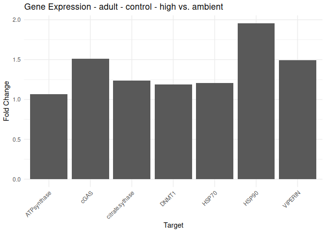
9.2.2 Life stage comparisons
# Generate bar plots for each group of comparison
plot_list <- fold_change_life_stage_df %>%
  split(.$comparison) %>%
  lapply(function(df) {
    comparison_title <- gsub("delta_delta_Cq_", "", unique(df$comparison))
    comparison_title <- gsub("_vs_", " vs. ", comparison_title)
    ggplot(df, aes(x = Target, y = fold_change)) +
      geom_bar(stat = "identity") +
      labs(title = paste("Gene Expression -", comparison_title), x = "Target", y = "Fold Change") +
      theme_minimal() +
      theme(axis.text.x = element_text(angle = 45, hjust = 1))
  })

# Display the plots
for (plot in plot_list) {
  print(plot)
}
9.2.3 Conditioning comparisons

9.2.4 Line plot conditioning comparisons across lifestages
9.2.5 Acute treatment comparison
10 Running linear models
10.1 ANOVA models
hist(delta_Cq_df$delta_Cq)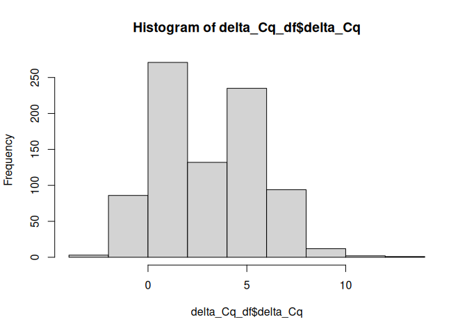
Run an anova model to test for effects of lifestage, conditioning, and acute treatment on delta Cq values for each target.
10.1.1 ATP synthase
ATP synthase is an enzyme complex that functions to synthesize adenosine triphosphate (ATP) from adenosine diphosphate (ADP) and inorganic phosphate (Pi), essentially generating the cell’s primary energy currency by harnessing the energy from a proton gradient across a membrane.
library(car)
library(emmeans)

model<-delta_Cq_df%>%
  filter(Target=="ATPsynthase")%>%

  aov(delta_Cq ~ life.stage * conditioning.treatment * acute.treatment, data=.)

summary(model)
Df Sum Sq Mean Sq F value
life.stage 3 2.66 0.8874 2.360
conditioning.treatment 1 1.33 1.3317 3.542
acute.treatment 1 0.61 0.6073 1.615
life.stage:conditioning.treatment 3 0.60 0.2012 0.535
life.stage:acute.treatment 3 0.37 0.1221 0.325
conditioning.treatment:acute.treatment 1 0.11 0.1095 0.291
life.stage:conditioning.treatment:acute.treatment 3 0.48 0.1591 0.423
Residuals 104 39.10 0.3760
Pr(>F)
life.stage 0.0757 .
conditioning.treatment 0.0626 .
acute.treatment 0.2066
life.stage:conditioning.treatment 0.6592
life.stage:acute.treatment 0.8074
conditioning.treatment:acute.treatment 0.5906
life.stage:conditioning.treatment:acute.treatment 0.7367
Residuals
---
Signif. codes: 0 '***' 0.001 '**' 0.01 '*' 0.05 '.' 0.1 ' ' 1qqPlot(model$residuals)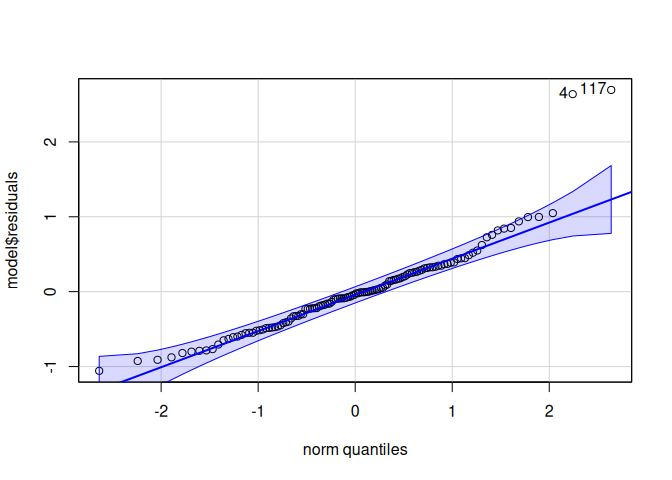
[1] 117 4leveneTest(model$residuals ~ life.stage*conditioning.treatment*acute.treatment, data=delta_Cq_df%>%filter(Target=="ATPsynthase"))Levene's Test for Homogeneity of Variance (center = median)
Df F value Pr(>F)
group 15 1.2733 0.2324
104 No significant effects.
10.1.2 DNMT1
The DNMT1 gene provides instructions for making an enzyme called DNA methyltransferase 1. This enzyme is involved in DNA methylation, which is the addition of methyl groups, consisting of one carbon atom and three hydrogen atoms, to DNA molecules.
model<-delta_Cq_df%>%
  filter(Target=="DNMT1")%>%

  aov(delta_Cq ~ life.stage * conditioning.treatment * acute.treatment, data=.)

summary(model)
Df Sum Sq Mean Sq F value
life.stage 3 1.47 0.490 0.347
conditioning.treatment 1 0.25 0.252 0.178
acute.treatment 1 2.88 2.885 2.041
life.stage:conditioning.treatment 3 10.35 3.451 2.442
life.stage:acute.treatment 3 4.53 1.511 1.069
conditioning.treatment:acute.treatment 1 0.01 0.011 0.008
life.stage:conditioning.treatment:acute.treatment 3 9.86 3.288 2.326
Residuals 102 144.16 1.413
Pr(>F)
life.stage 0.7915
conditioning.treatment 0.6736
acute.treatment 0.1561
life.stage:conditioning.treatment 0.0685 .
life.stage:acute.treatment 0.3657
conditioning.treatment:acute.treatment 0.9288
life.stage:conditioning.treatment:acute.treatment 0.0791 .
Residuals
---
Signif. codes: 0 '***' 0.001 '**' 0.01 '*' 0.05 '.' 0.1 ' ' 1qqPlot(model$residuals)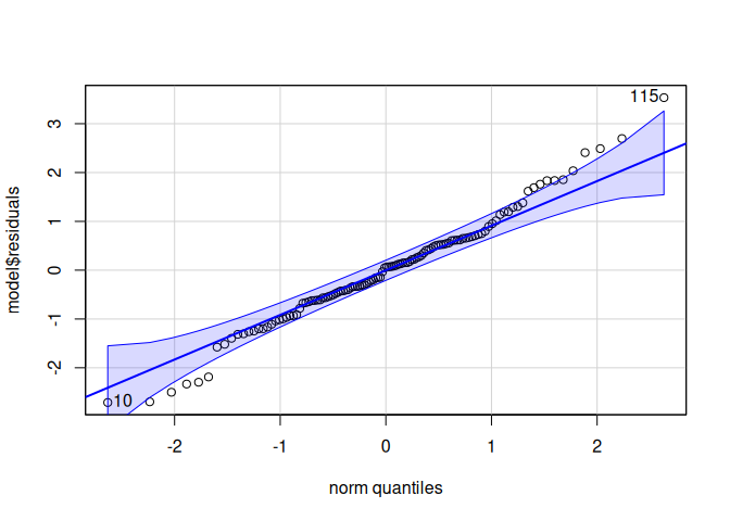
[1] 115 10leveneTest(model$residuals ~ life.stage*conditioning.treatment*acute.treatment, data=delta_Cq_df%>%filter(Target=="DNMT1"))Levene's Test for Homogeneity of Variance (center = median)
Df F value Pr(>F)
group 15 1.0926 0.3727
102 No significant effects.
10.1.3 HSP70
Heat Shock Protein 70 (Hsp70) is a molecular chaperone that plays crucial roles in maintaining cellular protein homeostasis and protecting cells from stress.
model<-delta_Cq_df%>%
  filter(Target=="HSP70")%>%

  aov(delta_Cq ~ life.stage * conditioning.treatment * acute.treatment, data=.)

summary(model)
Df Sum Sq Mean Sq F value
life.stage 3 23.4 7.814 2.464
conditioning.treatment 1 3.7 3.729 1.176
acute.treatment 1 2.1 2.136 0.674
life.stage:conditioning.treatment 3 14.2 4.735 1.493
life.stage:acute.treatment 3 14.9 4.966 1.566
conditioning.treatment:acute.treatment 1 19.0 18.966 5.980
life.stage:conditioning.treatment:acute.treatment 3 17.2 5.749 1.813
Residuals 104 329.8 3.172
Pr(>F)
life.stage 0.0666 .
conditioning.treatment 0.2807
acute.treatment 0.4137
life.stage:conditioning.treatment 0.2208
life.stage:acute.treatment 0.2022
conditioning.treatment:acute.treatment 0.0161 *
life.stage:conditioning.treatment:acute.treatment 0.1494
Residuals
---
Signif. codes: 0 '***' 0.001 '**' 0.01 '*' 0.05 '.' 0.1 ' ' 1qqPlot(model$residuals)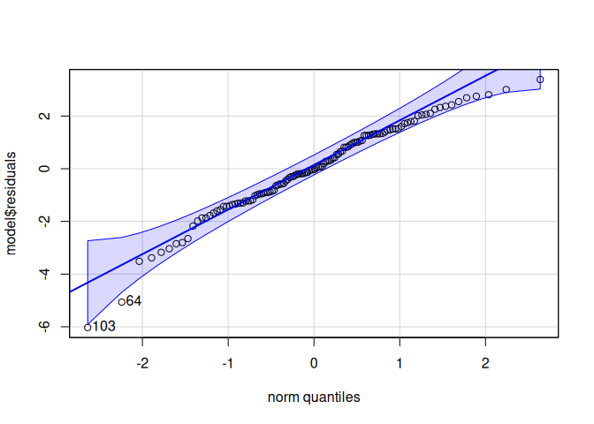
[1] 103 64leveneTest(model$residuals ~ life.stage*conditioning.treatment*acute.treatment, data=delta_Cq_df%>%filter(Target=="HSP70"))Levene's Test for Homogeneity of Variance (center = median)
Df F value Pr(>F)
group 15 0.5223 0.9231
104 emm<-emmeans(model, ~ conditioning.treatment:acute.treatment | life.stage)
pairs(emm)life.stage = adult:
contrast estimate SE df t.ratio p.value
control ambient - treated ambient -0.9455 0.890 104 -1.062 0.7134
control ambient - control high 0.2715 0.890 104 0.305 0.9901
control ambient - treated high -0.6649 0.890 104 -0.747 0.8779
treated ambient - control high 1.2170 0.890 104 1.367 0.5230
treated ambient - treated high 0.2806 0.890 104 0.315 0.9891
control high - treated high -0.9364 0.890 104 -1.052 0.7195
life.stage = juvenile:
contrast estimate SE df t.ratio p.value
control ambient - treated ambient -1.6377 0.939 104 -1.745 0.3061
control ambient - control high 0.1868 0.800 104 0.233 0.9955
control ambient - treated high 0.2839 0.840 104 0.338 0.9866
treated ambient - control high 1.8245 0.904 104 2.019 0.1878
treated ambient - treated high 1.9216 0.939 104 2.047 0.1776
control high - treated high 0.0971 0.800 104 0.121 0.9994
life.stage = seed:
contrast estimate SE df t.ratio p.value
control ambient - treated ambient -0.9181 0.818 104 -1.122 0.6769
control ambient - control high -1.4793 0.920 104 -1.608 0.3784
control ambient - treated high -1.2825 0.920 104 -1.395 0.5056
treated ambient - control high -0.5612 0.939 104 -0.598 0.9325
treated ambient - treated high -0.3644 0.939 104 -0.388 0.9800
control high - treated high 0.1967 1.030 104 0.191 0.9975
life.stage = spat:
contrast estimate SE df t.ratio p.value
control ambient - treated ambient -1.2358 1.080 104 -1.146 0.6620
control ambient - control high -1.8735 1.150 104 -1.630 0.3666
control ambient - treated high 1.4741 0.991 104 1.488 0.4485
treated ambient - control high -0.6376 1.190 104 -0.534 0.9506
treated ambient - treated high 2.7099 1.040 104 2.599 0.0516
control high - treated high 3.3475 1.120 104 2.999 0.0176
P value adjustment: tukey method for comparing a family of 4 estimates Significant effect of conditioning x acute treatment.
10.1.4 HSP90
Heat shock protein 90 (Hsp90) is a molecular chaperone that helps proteins fold, mature, and remain active. Hsp90 also helps regulate signaling networks and is involved in many cellular processes.
model<-delta_Cq_df%>%
  filter(Target=="HSP90")%>%

  aov(delta_Cq ~ life.stage * conditioning.treatment * acute.treatment, data=.)

summary(model)
Df Sum Sq Mean Sq F value
life.stage 3 27.25 9.083 13.042
conditioning.treatment 1 0.66 0.662 0.950
acute.treatment 1 17.57 17.570 25.230
life.stage:conditioning.treatment 3 5.61 1.870 2.686
life.stage:acute.treatment 3 3.89 1.298 1.864
conditioning.treatment:acute.treatment 1 1.09 1.088 1.562
life.stage:conditioning.treatment:acute.treatment 3 3.52 1.173 1.684
Residuals 104 72.43 0.696
Pr(>F)
life.stage 2.70e-07 ***
conditioning.treatment 0.3319
acute.treatment 2.12e-06 ***
life.stage:conditioning.treatment 0.0504 .
life.stage:acute.treatment 0.1402
conditioning.treatment:acute.treatment 0.2142
life.stage:conditioning.treatment:acute.treatment 0.1749
Residuals
---
Signif. codes: 0 '***' 0.001 '**' 0.01 '*' 0.05 '.' 0.1 ' ' 1qqPlot(model$residuals)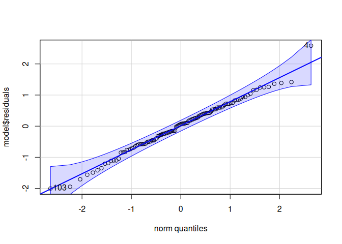
[1] 4 103leveneTest(model$residuals ~ life.stage*conditioning.treatment*acute.treatment, data=delta_Cq_df%>%filter(Target=="HSP90"))Levene's Test for Homogeneity of Variance (center = median)
Df F value Pr(>F)
group 15 1.1241 0.3447
104 emm<-emmeans(model, ~ conditioning.treatment:acute.treatment | life.stage)
pairs(emm)life.stage = adult:
contrast estimate SE df t.ratio p.value
control ambient - treated ambient -0.2939 0.417 104 -0.704 0.8951
control ambient - control high 0.9690 0.417 104 2.322 0.0995
control ambient - treated high -0.2648 0.417 104 -0.635 0.9206
treated ambient - control high 1.2630 0.417 104 3.027 0.0162
treated ambient - treated high 0.0292 0.417 104 0.070 0.9999
control high - treated high -1.2338 0.417 104 -2.957 0.0198
life.stage = juvenile:
contrast estimate SE df t.ratio p.value
control ambient - treated ambient 0.3117 0.440 104 0.709 0.8935
control ambient - control high 0.9955 0.375 104 2.654 0.0448
control ambient - treated high 0.8158 0.393 104 2.074 0.1686
treated ambient - control high 0.6838 0.424 104 1.614 0.3750
treated ambient - treated high 0.5041 0.440 104 1.146 0.6619
control high - treated high -0.1797 0.375 104 -0.479 0.9636
life.stage = seed:
contrast estimate SE df t.ratio p.value
control ambient - treated ambient -0.0352 0.383 104 -0.092 0.9997
control ambient - control high 0.7954 0.431 104 1.846 0.2581
control ambient - treated high 0.0628 0.431 104 0.146 0.9989
treated ambient - control high 0.8307 0.440 104 1.889 0.2392
treated ambient - treated high 0.0981 0.440 104 0.223 0.9961
control high - treated high -0.7326 0.482 104 -1.520 0.4290
life.stage = spat:
contrast estimate SE df t.ratio p.value
control ambient - treated ambient -0.1549 0.505 104 -0.306 0.9900
control ambient - control high 0.8926 0.539 104 1.657 0.3516
control ambient - treated high 1.7849 0.464 104 3.845 0.0012
treated ambient - control high 1.0475 0.560 104 1.871 0.2468
treated ambient - treated high 1.9398 0.489 104 3.970 0.0008
control high - treated high 0.8923 0.523 104 1.706 0.3258
P value adjustment: tukey method for comparing a family of 4 estimates Significant effect of lifestage x acute treatment, lifestage x conditioning treatment, acute treatment, and lifestage.
10.1.5 cGAS
The cGAS gene is involved in several processes, including cellular response to exogenous dsRNA, positive regulation of intracellular signal transduction, and regulation of defense response.
model<-delta_Cq_df%>%
  filter(Target=="cGAS")%>%

  aov(delta_Cq ~ life.stage * conditioning.treatment * acute.treatment, data=.)

summary(model)
Df Sum Sq Mean Sq F value
life.stage 3 5.64 1.881 1.302
conditioning.treatment 1 0.55 0.545 0.377
acute.treatment 1 2.43 2.429 1.681
life.stage:conditioning.treatment 3 1.32 0.440 0.305
life.stage:acute.treatment 3 12.86 4.286 2.965
conditioning.treatment:acute.treatment 1 0.31 0.311 0.215
life.stage:conditioning.treatment:acute.treatment 3 4.65 1.550 1.073
Residuals 104 150.32 1.445
Pr(>F)
life.stage 0.2779
conditioning.treatment 0.5404
acute.treatment 0.1977
life.stage:conditioning.treatment 0.8220
life.stage:acute.treatment 0.0355 *
conditioning.treatment:acute.treatment 0.6436
life.stage:conditioning.treatment:acute.treatment 0.3641
Residuals
---
Signif. codes: 0 '***' 0.001 '**' 0.01 '*' 0.05 '.' 0.1 ' ' 1qqPlot(model$residuals)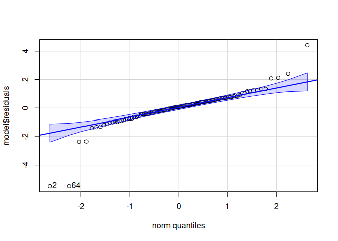
[1] 2 64leveneTest(model$residuals ~ life.stage*conditioning.treatment*acute.treatment, data=delta_Cq_df%>%filter(Target=="cGAS"))Levene's Test for Homogeneity of Variance (center = median)
Df F value Pr(>F)
group 15 1.5918 0.08854 .
104
---
Signif. codes: 0 '***' 0.001 '**' 0.01 '*' 0.05 '.' 0.1 ' ' 1emm<-emmeans(model, ~ conditioning.treatment:acute.treatment | life.stage)
pairs(emm)life.stage = adult:
contrast estimate SE df t.ratio p.value
control ambient - treated ambient 0.0739 0.601 104 0.123 0.9993
control ambient - control high 0.5983 0.601 104 0.995 0.7524
control ambient - treated high 0.1334 0.601 104 0.222 0.9961
treated ambient - control high 0.5244 0.601 104 0.872 0.8191
treated ambient - treated high 0.0595 0.601 104 0.099 0.9996
control high - treated high -0.4649 0.601 104 -0.773 0.8663
life.stage = juvenile:
contrast estimate SE df t.ratio p.value
control ambient - treated ambient 0.3421 0.634 104 0.540 0.9490
control ambient - control high -0.1441 0.540 104 -0.267 0.9933
control ambient - treated high 0.0553 0.567 104 0.098 0.9997
treated ambient - control high -0.4862 0.610 104 -0.797 0.8557
treated ambient - treated high -0.2869 0.634 104 -0.453 0.9690
control high - treated high 0.1994 0.540 104 0.369 0.9828
life.stage = seed:
contrast estimate SE df t.ratio p.value
control ambient - treated ambient 0.1936 0.552 104 0.350 0.9852
control ambient - control high -1.5259 0.621 104 -2.458 0.0728
control ambient - treated high -1.0451 0.621 104 -1.683 0.3376
treated ambient - control high -1.7195 0.634 104 -2.714 0.0384
treated ambient - treated high -1.2387 0.634 104 -1.955 0.2120
control high - treated high 0.4808 0.694 104 0.693 0.8997
life.stage = spat:
contrast estimate SE df t.ratio p.value
control ambient - treated ambient -0.6338 0.728 104 -0.871 0.8200
control ambient - control high -0.8533 0.776 104 -1.100 0.6906
control ambient - treated high 0.2963 0.669 104 0.443 0.9708
treated ambient - control high -0.2195 0.806 104 -0.272 0.9929
treated ambient - treated high 0.9301 0.704 104 1.321 0.5516
control high - treated high 1.1496 0.754 104 1.526 0.4260
P value adjustment: tukey method for comparing a family of 4 estimates Significant effect of lifestage x acute treatment and lifestage.
10.1.6 Citrate synthase
Citrate synthase is important for energy production in the TCA cycle and is linked to the electron transport chain. It is also used as an enzyme marker for intact mitochondria.
model<-delta_Cq_df%>%
  filter(Target=="citrate synthase")%>%

  aov(delta_Cq ~ life.stage * conditioning.treatment * acute.treatment, data=.)

summary(model)
Df Sum Sq Mean Sq F value
life.stage 3 10.15 3.383 6.975
conditioning.treatment 1 1.31 1.305 2.692
acute.treatment 1 6.78 6.777 13.975
life.stage:conditioning.treatment 3 0.47 0.158 0.325
life.stage:acute.treatment 3 7.74 2.580 5.320
conditioning.treatment:acute.treatment 1 1.10 1.104 2.276
life.stage:conditioning.treatment:acute.treatment 3 0.13 0.045 0.092
Residuals 104 50.43 0.485
Pr(>F)
life.stage 0.000254 ***
conditioning.treatment 0.103872
acute.treatment 0.000303 ***
life.stage:conditioning.treatment 0.807157
life.stage:acute.treatment 0.001888 **
conditioning.treatment:acute.treatment 0.134455
life.stage:conditioning.treatment:acute.treatment 0.964379
Residuals
---
Signif. codes: 0 '***' 0.001 '**' 0.01 '*' 0.05 '.' 0.1 ' ' 1qqPlot(model$residuals)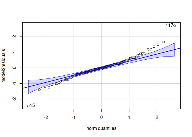
[1] 117 15leveneTest(model$residuals ~ life.stage*conditioning.treatment*acute.treatment, data=delta_Cq_df%>%filter(Target=="citrate synthase"))Levene's Test for Homogeneity of Variance (center = median)
Df F value Pr(>F)
group 15 2.0302 0.01964 *
104
---
Signif. codes: 0 '***' 0.001 '**' 0.01 '*' 0.05 '.' 0.1 ' ' 1emm<-emmeans(model, ~ conditioning.treatment:acute.treatment | life.stage)
pairs(emm)life.stage = adult:
contrast estimate SE df t.ratio p.value
control ambient - treated ambient 0.31754 0.348 104 0.912 0.7985
control ambient - control high 0.30936 0.348 104 0.888 0.8108
control ambient - treated high 0.14178 0.348 104 0.407 0.9771
treated ambient - control high -0.00818 0.348 104 -0.023 1.0000
treated ambient - treated high -0.17576 0.348 104 -0.505 0.9578
control high - treated high -0.16758 0.348 104 -0.481 0.9631
life.stage = juvenile:
contrast estimate SE df t.ratio p.value
control ambient - treated ambient 0.69618 0.367 104 1.897 0.2357
control ambient - control high 0.08720 0.313 104 0.279 0.9924
control ambient - treated high 0.25576 0.328 104 0.779 0.8638
treated ambient - control high -0.60898 0.353 104 -1.723 0.3170
treated ambient - treated high -0.44042 0.367 104 -1.200 0.6282
control high - treated high 0.16856 0.313 104 0.539 0.9494
life.stage = seed:
contrast estimate SE df t.ratio p.value
control ambient - treated ambient 0.36475 0.320 104 1.140 0.6657
control ambient - control high -0.97515 0.360 104 -2.712 0.0386
control ambient - treated high -0.88377 0.360 104 -2.458 0.0728
treated ambient - control high -1.33990 0.367 104 -3.651 0.0023
treated ambient - treated high -1.24852 0.367 104 -3.402 0.0052
control high - treated high 0.09138 0.402 104 0.227 0.9958
life.stage = spat:
contrast estimate SE df t.ratio p.value
control ambient - treated ambient 0.37761 0.422 104 0.895 0.8072
control ambient - control high -0.89118 0.450 104 -1.983 0.2012
control ambient - treated high -0.70657 0.387 104 -1.824 0.2681
treated ambient - control high -1.26879 0.467 104 -2.716 0.0382
treated ambient - treated high -1.08418 0.408 104 -2.659 0.0443
control high - treated high 0.18460 0.436 104 0.423 0.9744
P value adjustment: tukey method for comparing a family of 4 estimates Significant effect of acute treatment and lifestage x acute treatment.
10.1.7 Viperin
Viperin limits replication of DNA and RNA viruses.
model<-delta_Cq_df%>%
  filter(Target=="viperin")%>%

  aov(delta_Cq ~ life.stage * conditioning.treatment * acute.treatment, data=.)

summary(model)
Df Sum Sq Mean Sq F value
life.stage 3 91.90 30.635 15.749
conditioning.treatment 1 2.08 2.080 1.069
acute.treatment 1 0.76 0.760 0.391
life.stage:conditioning.treatment 3 9.03 3.011 1.548
life.stage:acute.treatment 3 8.58 2.861 1.471
conditioning.treatment:acute.treatment 1 2.01 2.010 1.033
life.stage:conditioning.treatment:acute.treatment 3 0.94 0.313 0.161
Residuals 102 198.41 1.945
Pr(>F)
life.stage 1.73e-08 ***
conditioning.treatment 0.304
acute.treatment 0.533
life.stage:conditioning.treatment 0.207
life.stage:acute.treatment 0.227
conditioning.treatment:acute.treatment 0.312
life.stage:conditioning.treatment:acute.treatment 0.922
Residuals
---
Signif. codes: 0 '***' 0.001 '**' 0.01 '*' 0.05 '.' 0.1 ' ' 1qqPlot(model$residuals)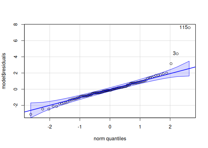
[1] 115 3leveneTest(model$residuals ~ life.stage*conditioning.treatment*acute.treatment, data=delta_Cq_df%>%filter(Target=="viperin"))Levene's Test for Homogeneity of Variance (center = median)
Df F value Pr(>F)
group 15 1.4856 0.1245
102 emm<-emmeans(model, ~ conditioning.treatment:acute.treatment | life.stage)
pairs(emm)life.stage = adult:
contrast estimate SE df t.ratio p.value
control ambient - treated ambient 0.1683 0.697 102 0.241 0.9950
control ambient - control high 0.5763 0.697 102 0.826 0.8418
control ambient - treated high 0.2376 0.697 102 0.341 0.9863
treated ambient - control high 0.4081 0.697 102 0.585 0.9363
treated ambient - treated high 0.0693 0.697 102 0.099 0.9996
control high - treated high -0.3388 0.697 102 -0.486 0.9621
life.stage = juvenile:
contrast estimate SE df t.ratio p.value
control ambient - treated ambient 1.5727 0.735 102 2.140 0.1477
control ambient - control high 0.6795 0.627 102 1.084 0.7001
control ambient - treated high 1.2753 0.657 102 1.940 0.2181
treated ambient - control high -0.8932 0.708 102 -1.262 0.5892
treated ambient - treated high -0.2974 0.735 102 -0.405 0.9775
control high - treated high 0.5958 0.627 102 0.950 0.7777
life.stage = seed:
contrast estimate SE df t.ratio p.value
control ambient - treated ambient -0.1371 0.678 102 -0.202 0.9971
control ambient - control high -0.5242 0.735 102 -0.713 0.8917
control ambient - treated high -1.1583 0.735 102 -1.576 0.3970
treated ambient - control high -0.3872 0.753 102 -0.514 0.9556
treated ambient - treated high -1.0212 0.753 102 -1.356 0.5298
control high - treated high -0.6341 0.805 102 -0.787 0.8600
life.stage = spat:
contrast estimate SE df t.ratio p.value
control ambient - treated ambient 0.5456 0.845 102 0.646 0.9167
control ambient - control high -0.9091 0.900 102 -1.010 0.7440
control ambient - treated high -0.2650 0.776 102 -0.341 0.9862
treated ambient - control high -1.4547 0.936 102 -1.555 0.4090
treated ambient - treated high -0.8105 0.817 102 -0.993 0.7540
control high - treated high 0.6442 0.874 102 0.737 0.8820
P value adjustment: tukey method for comparing a family of 4 estimates Significant effect of acute treatment and lifestage x acute treatment.
All tests pass normality and homogeneity of variance. ANOVA tests are appropriate.
10.2 Plotting
Display plot of acute x conditioning treatment faceted for each lifestage for each target.
Show sample size for each group.
delta_Cq_df%>%
  group_by(life.stage, acute.treatment, conditioning.treatment)%>%
  summarise(n=length(unique(Sample)))
# A tibble: 16 × 4
# Groups: life.stage, acute.treatment [8]
life.stage acute.treatment conditioning.treatment n
<chr> <chr> <chr> <int>
1 adult ambient control 8
2 adult ambient treated 8
3 adult high control 8
4 adult high treated 8
5 juvenile ambient control 9
6 juvenile ambient treated 6
7 juvenile high control 11
8 juvenile high treated 9
9 seed ambient control 10
10 seed ambient treated 9
11 seed high control 6
12 seed high treated 6
13 spat ambient control 6
14 spat ambient treated 5
15 spat high control 4
16 spat high treated 7Note that sample sizes for spat, seed, or juveniles that are <6 are due to lack of RNA isolated from the samples.
Adults were all sampled from one family (Pink). Previous flow cytometry was unclear as to diploid or triploid classification. We have extracted DNA that we can use to verify ploidy.
10.2.1 ATP synthase: No effects
plot1<-delta_Cq_df%>%
  filter(Target=="ATPsynthase")%>%

  group_by(Target, life.stage, acute.treatment, conditioning.treatment)%>%
  summarise(mean=mean(delta_Cq, na.rm=TRUE), se=sd(delta_Cq, na.rm=TRUE)/sqrt(length(delta_Cq)))%>%

  ggplot(aes(x=acute.treatment, y=mean, colour=conditioning.treatment))+
  facet_grid(~life.stage)+
  scale_colour_manual(values=c("darkgray", "orange"))+
  geom_point()+
  geom_line(aes(group=conditioning.treatment))+
  geom_errorbar(aes(ymin=mean-se, ymax=mean+se), width=0.1)+
  ggtitle("ATP synthase (no sign. effects)")+
  ylab("Delta Cq")+
  ylim(-0.5,1.5)+
  geom_hline(yintercept=0, linetype="dashed")+
  theme_classic();plot1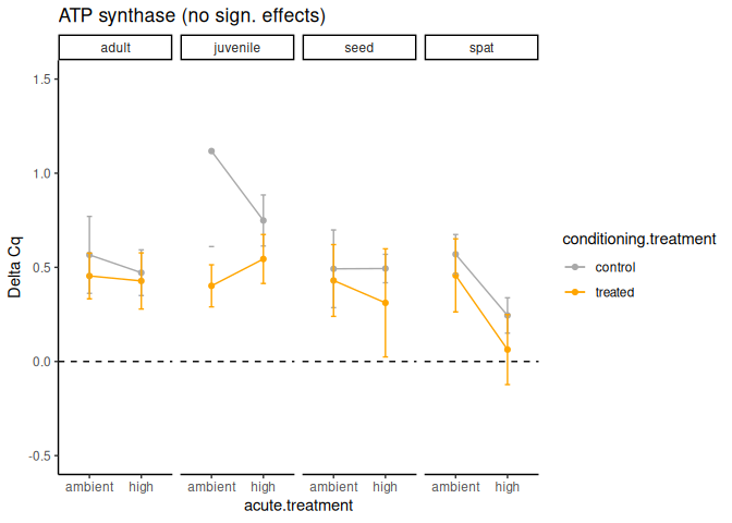
10.2.2 DNMT1: No effects
plot2<-delta_Cq_df%>%
  filter(Target=="DNMT1")%>%

  group_by(Target, life.stage, acute.treatment, conditioning.treatment)%>%
  summarise(mean=mean(delta_Cq, na.rm=TRUE), se=sd(delta_Cq, na.rm=TRUE)/sqrt(length(delta_Cq)))%>%

  ggplot(aes(x=acute.treatment, y=mean, colour=conditioning.treatment))+
  facet_grid(~life.stage)+
  geom_point()+
  scale_colour_manual(values=c("darkgray", "orange"))+
  geom_line(aes(group=conditioning.treatment))+
  geom_errorbar(aes(ymin=mean-se, ymax=mean+se), width=0.1)+
  ggtitle("DMNT1 (no sign. effects)")+
  ylab("Delta Cq")+
  geom_hline(yintercept=0, linetype="dashed")+
  ylim(0,9)+
  theme_classic();plot2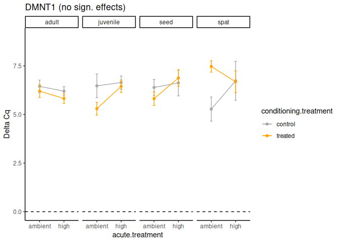
10.2.3 HSP70: Significant effect of conditioning x acute treatment.
plot3<-delta_Cq_df%>%
  filter(Target=="HSP70")%>%

  group_by(Target, life.stage, acute.treatment, conditioning.treatment)%>%
  summarise(mean=mean(delta_Cq, na.rm=TRUE), se=sd(delta_Cq, na.rm=TRUE)/sqrt(length(delta_Cq)))%>%

  ggplot(aes(x=acute.treatment, y=mean, colour=conditioning.treatment))+
  facet_grid(~life.stage)+
  scale_colour_manual(values=c("darkgray", "orange"))+
  geom_point()+
  geom_line(aes(group=conditioning.treatment))+
  geom_errorbar(aes(ymin=mean-se, ymax=mean+se), width=0.1)+
  ggtitle("HSP70  (sign. conditioning x acute treatment)")+
  ylab("Delta Cq")+
  ylim(0,8)+
  geom_hline(yintercept=0, linetype="dashed")+
  theme_classic();plot3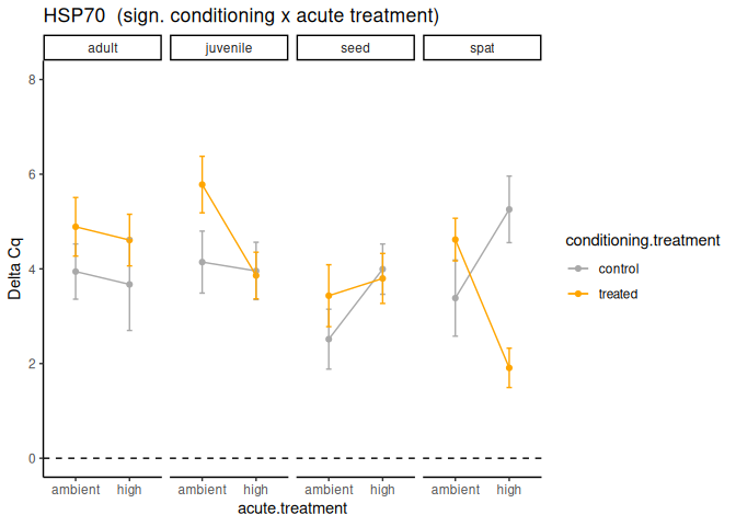
plot3a<-delta_Cq_df%>%
  filter(Target=="HSP70")%>%

  group_by(Target, acute.treatment, conditioning.treatment)%>%
  summarise(mean=mean(delta_Cq, na.rm=TRUE), se=sd(delta_Cq, na.rm=TRUE)/sqrt(length(delta_Cq)))%>%

  ggplot(aes(x=acute.treatment, y=mean, colour=conditioning.treatment))+
  geom_point()+
  scale_colour_manual(values=c("darkgray", "orange"))+
  geom_line(aes(group=conditioning.treatment))+
  geom_errorbar(aes(ymin=mean-se, ymax=mean+se), width=0.1)+
  ggtitle("HSP70  (sign. conditioning x acute treatment)")+
  ylab("Delta Cq")+
  geom_hline(yintercept=0, linetype="dashed")+
  ylim(0,8)+
  theme_classic();plot3a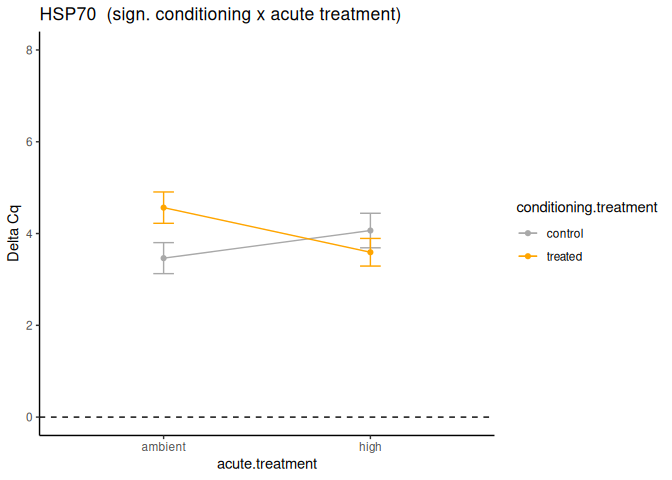
10.2.4 HSP90: Significant effect of lifestage x acute treatment, lifestage x conditioning treatment, acute treatment, and lifestage.
plot4<-delta_Cq_df%>%
  filter(Target=="HSP90")%>%

  group_by(Target, life.stage, acute.treatment, conditioning.treatment)%>%
  summarise(mean=mean(delta_Cq, na.rm=TRUE), se=sd(delta_Cq, na.rm=TRUE)/sqrt(length(delta_Cq)))%>%

  ggplot(aes(x=acute.treatment, y=mean, colour=conditioning.treatment))+
  facet_grid(~life.stage)+
  scale_colour_manual(values=c("darkgray", "orange"))+
  geom_point()+
  geom_line(aes(group=conditioning.treatment))+
  geom_errorbar(aes(ymin=mean-se, ymax=mean+se), width=0.1)+
  ggtitle("HSP90  (sign. lifestage x acute & lifestage x conditioning treatment)")+
  ylab("Delta Cq")+
  ylim(-2,2.5)+
  geom_hline(yintercept=0, linetype="dashed")+
  theme_classic();plot4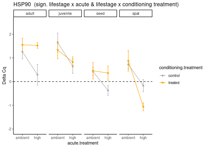
10.2.5 cGAS: Significant effect of lifestage x acute treatment and lifestage.
plot5<-delta_Cq_df%>%
  filter(Target=="cGAS")%>%

  group_by(Target, life.stage, acute.treatment, conditioning.treatment)%>%
  summarise(mean=mean(delta_Cq, na.rm=TRUE), se=sd(delta_Cq, na.rm=TRUE)/sqrt(length(delta_Cq)))%>%

  ggplot(aes(x=acute.treatment, y=mean, colour=conditioning.treatment))+
  facet_grid(~life.stage)+
  scale_colour_manual(values=c("darkgray", "orange"))+
  geom_point()+
  geom_line(aes(group=conditioning.treatment))+
  geom_errorbar(aes(ymin=mean-se, ymax=mean+se), width=0.1)+
  ggtitle("cGAS  (sign. lifestage x acute treatment)")+
  ylab("Delta Cq")+
  ylim(2,8)+
  geom_hline(yintercept=0, linetype="dashed")+
  theme_classic();plot5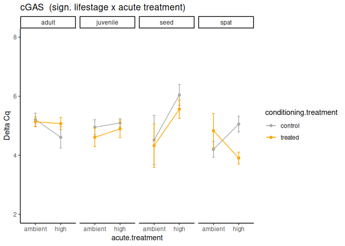
10.2.6 Citrate synthase: Significant effect of acute treatment and lifestage x acute treatment.
plot6<-delta_Cq_df%>%
  filter(Target=="citrate synthase")%>%

  group_by(Target, life.stage, acute.treatment, conditioning.treatment)%>%
  summarise(mean=mean(delta_Cq, na.rm=TRUE), se=sd(delta_Cq, na.rm=TRUE)/sqrt(length(delta_Cq)))%>%

  ggplot(aes(x=acute.treatment, y=mean, colour=conditioning.treatment))+
  facet_grid(~life.stage)+
  scale_colour_manual(values=c("darkgray", "orange"))+
  geom_point()+
  geom_line(aes(group=conditioning.treatment))+
  geom_errorbar(aes(ymin=mean-se, ymax=mean+se), width=0.1)+
  ggtitle("cGAS  (sign. lifestage x acute treatment)")+
  ylab("Delta Cq")+
  ylim(-2,3)+
  geom_hline(yintercept=0, linetype="dashed")+
  theme_classic();plot6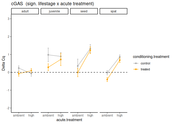
10.2.7 Viperin: Significant effect of lifestage and lifestage x acute treatment.
plot7<-delta_Cq_df%>%
  filter(Target=="viperin")%>%

  group_by(Target, life.stage, acute.treatment, conditioning.treatment)%>%
  summarise(mean=mean(delta_Cq, na.rm=TRUE), se=sd(delta_Cq, na.rm=TRUE)/sqrt(length(delta_Cq)))%>%

  ggplot(aes(x=acute.treatment, y=mean, colour=conditioning.treatment))+
  facet_grid(~life.stage)+
  scale_colour_manual(values=c("darkgray", "orange"))+
  geom_point()+
  geom_line(aes(group=conditioning.treatment))+
  geom_errorbar(aes(ymin=mean-se, ymax=mean+se), width=0.1)+
  ggtitle("Viperin  (sign. lifestage x acute treatment)")+
  ylab("Delta Cq")+
  ylim(0,6)+
  geom_hline(yintercept=0, linetype="dashed")+
  theme_classic();plot7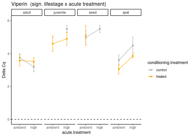
Plot spat HSP 70 and HSP 90
plot8<-delta_Cq_df%>%
  dplyr::filter(Target=="HSP90")%>%
  dplyr::filter(life.stage=="spat")%>%

  ggplot(aes(x=acute.treatment, y=delta_Cq, colour=conditioning.treatment))+
  facet_wrap(~Target, scales="free")+
  scale_colour_manual(values=c("darkgray", "orange"), name="Priming")+
  geom_boxplot(outliers=FALSE)+
  geom_point(position=position_jitterdodge(0.1))+
  ggtitle("HSP90")+
  geom_text(x=2, y=1, label="*", size=12, color="black")+
  ylab("Expression")+
  xlab("Temperature")+
  ylim(-2,3)+
  theme_classic()+
  theme(legend.position="none");plot8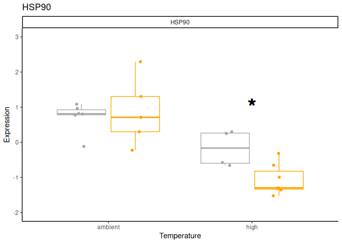
plot8a<-delta_Cq_df%>%
  dplyr::filter(Target=="HSP70")%>%
  dplyr::filter(life.stage=="spat")%>%

  ggplot(aes(x=acute.treatment, y=delta_Cq, colour=conditioning.treatment))+
  facet_wrap(~Target, scales="free")+
  scale_colour_manual(values=c("darkgray", "orange"), name="Priming")+
  geom_boxplot(outliers=FALSE)+
  geom_point(position=position_jitterdodge(0.1))+
  ggtitle("HSP70")+
  geom_text(x=2, y=9, label="*", size=12, color="black")+
  ylab("Expression")+
  xlab("Temperature")+
  ylim(-2,10)+
  theme_classic();plot8a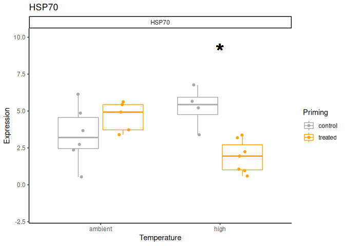
library(cowplot)
plots<-plot_grid(plot8, plot8a, nrow=1, rel_widths=c(0.8,1))

ggsave(plots, filename="../output/qPCR/spat-heat-shock.png", width=8, height=4)
10.3 Conclusions
10.3.1 Effects of conditioning on acute stress response
- HSP70 and 90 genes are affected by conditioning.
- HSP90 has significantly higher expression in treated adults than control adults at elevated temperature. No other lifestages have significant differences in expression between conditioning treatments at high temperature.
- HSP70 has significantly lower expression in treated spat than control spat at elevated temperature. No other lifestages have significant differences between conditioning treatments at high temperature.
10.3.2 Effects of acute stress and lifestage
- Across lifestages (except for juveniles) HSP90 decreases in expression under elevated temperature.
- Expression of cGAS increases most dramatically in seed under elevated temperature.
- ATP synthase and DMNT1 are not affected by elevated temperature.
- Citrate synthase increases in expression in seed and spat under elevated temperature, but does not change in adult or juvenile stages.
- Effects of acute treatment and life stage are just barely not significant for ATPsynthase and DMNT1. It is particularly interesting to see the trend for higher DMNT1 expression in spat at ambient temperature. There is also a trend for lower expression of ATPsynthase in seed at high temperature, but not technically significant.