INTRO
This continues development of the Summer Oyster Resilience & Mortality Index (SORMI) (SORMI website). M.gigas oysters from nine different USDA families, which were previously heat stressed @ 36oC and assessed by the resazurin assay on 20260415 (GitHub README), were subjected to a second heat stress.
Repo for this experiment is here:
MATERIALS & METHODS
Oysters were submered in ~100mL of Instant Ocean (25ppt salinity) in clear, plastic cups. They were held at 33oC and periodically assessed for mortality.
After the first day of heat stress, I believe Steven turned the incubator off overnight, due to his concern that too many oysters would die during a period in which no one would be available to check on them.
The text below is knitted from 00.00-mgig-heat-survivorship.Rmd.
1 BACKGROUND
This is a Kaplan-Meier survival analysis of 33oC heat stress of Magallana gigas oysters, conducted on 20260427 (GitHub repo). It compares 9 different families bred/selected by the USDA.
These oysters had been previously heat stressed @ 36oC and assessed by the resazurin assay on 20260415 (GitHub README)
1.1 SETUP
1.1.1 Load packages
library(readr)
library(dplyr)
library(survival)
library(ggplot2)

knitr::opts_chunk$set(
  echo = TRUE,         # Display code chunks
  eval = TRUE,        # Evaluate code chunks
  warning = FALSE,     # Hide warnings
  message = FALSE,     # Hide messages
  comment = "",         # Prevents appending '##' to beginning of lines in code output
  results = 'hold'     # Holds output so it's all printed together after code chunk
)
1.1.2 Read in and view raw data
survivorship_raw <- read_csv(
    "../heat-survivorship/20260427-33C-USDA-families/survivorship.csv",
    show_col_types = FALSE
)

# Preview newly created object
cat("\n=== survivorship_raw: str() ===\n")
str(survivorship_raw)
=== survivorship_raw: str() ===
spc_tbl_ [1,920 × 10] (S3: spec_tbl_df/tbl_df/tbl/data.frame)
$ individual_id : num [1:1920] 184 199 207 206 205 204 203 202 201 198 ...
$ familly_id.group : num [1:1920] 1 1 1 1 1 1 1 1 1 1 ...
$ timepoint_count : num [1:1920] 0 0 0 0 0 0 0 0 0 0 ...
$ timepoint_hrs : num [1:1920] 0 0 0 0 0 0 0 0 0 0 ...
$ alive.measurement : logi [1:1920] TRUE TRUE TRUE TRUE TRUE TRUE ...
$ date : Date[1:1920], format: "2026-04-27" "2026-04-27" ...
$ time : 'hms' num [1:1920] 11:30:00 11:30:00 11:30:00 11:30:00 ...
..- attr(*, "units")= chr "secs"
$ area_mm2.measurment: num [1:1920] 893 752 867 966 671 ...
$ imageJ_ID : logi [1:1920] NA NA NA NA NA NA ...
$ notes : chr [1:1920] NA NA NA NA ...
- attr(*, "spec")=
.. cols(
.. individual_id = col_double(),
.. familly_id.group = col_double(),
.. timepoint_count = col_double(),
.. timepoint_hrs = col_double(),
.. alive.measurement = col_logical(),
.. date = col_date(format = ""),
.. time = col_time(format = ""),
.. area_mm2.measurment = col_double(),
.. imageJ_ID = col_logical(),
.. notes = col_character()
.. )
- attr(*, "problems")=<pointer: 0x561a2453d570> 1.2 ANALYSIS
1.2.1 Clean and standardize columns used for survival analysis
survivorship_clean <- survivorship_raw %>%
    mutate(
        individual_id = as.character(individual_id),
        family_group = as.character(`familly_id.group`),
        timepoint_hrs = as.numeric(timepoint_hrs),
        alive_chr = toupper(trimws(as.character(`alive.measurement`))),
        alive = case_when(
            alive_chr %in% c("TRUE", "T", "1", "YES", "Y") ~ TRUE,
            alive_chr %in% c("FALSE", "F", "0", "NO", "N") ~ FALSE,
            TRUE ~ NA
        )
    ) %>%
    select(
        individual_id,
        family_group,
        timepoint_count,
        timepoint_hrs,
        alive,
        date,
        time,
        everything()
    )

# Preview newly created object
cat("\n=== survivorship_clean: str() ===\n")
str(survivorship_clean)
cat("\n=== survivorship_clean: summary(alive) ===\n")
summary(survivorship_clean$alive)
=== survivorship_clean: str() ===
tibble [1,920 × 13] (S3: tbl_df/tbl/data.frame)
$ individual_id : chr [1:1920] "184" "199" "207" "206" ...
$ family_group : chr [1:1920] "1" "1" "1" "1" ...
$ timepoint_count : num [1:1920] 0 0 0 0 0 0 0 0 0 0 ...
$ timepoint_hrs : num [1:1920] 0 0 0 0 0 0 0 0 0 0 ...
$ alive : logi [1:1920] TRUE TRUE TRUE TRUE TRUE TRUE ...
$ date : Date[1:1920], format: "2026-04-27" "2026-04-27" ...
$ time : 'hms' num [1:1920] 11:30:00 11:30:00 11:30:00 11:30:00 ...
..- attr(*, "units")= chr "secs"
$ familly_id.group : num [1:1920] 1 1 1 1 1 1 1 1 1 1 ...
$ alive.measurement : logi [1:1920] TRUE TRUE TRUE TRUE TRUE TRUE ...
$ area_mm2.measurment: num [1:1920] 893 752 867 966 671 ...
$ imageJ_ID : logi [1:1920] NA NA NA NA NA NA ...
$ notes : chr [1:1920] NA NA NA NA ...
$ alive_chr : chr [1:1920] "TRUE" "TRUE" "TRUE" "TRUE" ...
=== survivorship_clean: summary(alive) ===
Mode FALSE TRUE
logical 281 1639 1.2.2 Reduce repeated observations to one survival row per individual
individual_survival <- survivorship_clean %>%
    filter(!is.na(individual_id), !is.na(timepoint_hrs), !is.na(alive)) %>%
    arrange(individual_id, timepoint_hrs) %>%
    group_by(individual_id) %>%
    summarise(
        family_group = first(family_group[!is.na(family_group)]),
        event = if_else(any(!alive), 1L, 0L),
        time_to_event = {
            if (any(!alive)) {
                min(timepoint_hrs[!alive])
            } else {
                max(timepoint_hrs)
            }
        },
        n_observations = n(),
        .groups = "drop"
    )

# Preview newly created object
cat("\n=== individual_survival: str() ===\n")
str(individual_survival)
cat("\n=== individual_survival: summary(time_to_event) ===\n")
summary(individual_survival$time_to_event)
cat("\n=== individual_survival: table(event) ===\n")
table(individual_survival$event)
=== individual_survival: str() ===
tibble [128 × 5] (S3: tbl_df/tbl/data.frame)
$ individual_id : chr [1:128] "1" "101" "102" "103" ...
$ family_group : chr [1:128] "6" "9" "5" "3" ...
$ event : int [1:128] 0 0 0 1 0 0 0 1 0 1 ...
$ time_to_event : num [1:128] 99.5 99.5 99.5 93 99.5 99.5 99.5 99.5 99.5 93 ...
$ n_observations: int [1:128] 15 15 15 15 15 15 15 15 15 15 ...
=== individual_survival: summary(time_to_event) ===
Min. 1st Qu. Median Mean 3rd Qu. Max.
20.00 93.00 99.50 86.49 99.50 99.50
=== individual_survival: table(event) ===
0 1
65 63 1.2.3 Create Surv object and fit Kaplan-Meier models
surv_object <- with(individual_survival, Surv(time = time_to_event, event = event))

km_fit_overall <- survfit(surv_object ~ 1, data = individual_survival)
km_fit_by_family <- survfit(surv_object ~ family_group, data = individual_survival)

# Preview newly created objects
cat("\n=== km_fit_overall ===\n")
print(km_fit_overall)
cat("\n=== km_fit_by_family ===\n")
print(km_fit_by_family)
cat("\n=== km_fit_overall: str() ===\n")
str(km_fit_overall)
cat("\n=== km_fit_by_family: str() ===\n")
str(km_fit_by_family)
=== km_fit_overall ===
Call: survfit(formula = surv_object ~ 1, data = individual_survival)
n events median 0.95LCL 0.95UCL
[1,] 128 63 NA 96.5 NA
=== km_fit_by_family ===
Call: survfit(formula = surv_object ~ family_group, data = individual_survival)
n events median 0.95LCL 0.95UCL
family_group=1 20 12 93.0 52.5 NA
family_group=10 9 5 99.5 99.5 NA
family_group=2 8 3 NA 99.5 NA
family_group=3 20 8 NA 93.0 NA
family_group=5 20 8 NA 93.0 NA
family_group=6 9 4 NA 48.0 NA
family_group=7 17 10 96.5 69.5 NA
family_group=8 10 8 72.8 52.5 NA
family_group=9 15 5 NA 96.5 NA
=== km_fit_overall: str() ===
List of 17
$ n : int 128
$ time : num [1:9] 20 24 44 48 52.5 69.5 93 96.5 99.5
$ n.risk : num [1:9] 128 126 125 124 122 100 97 77 71
$ n.event : num [1:9] 2 1 1 2 22 3 20 6 6
$ n.censor : num [1:9] 0 0 0 0 0 0 0 0 65
$ surv : num [1:9] 0.984 0.977 0.969 0.953 0.781 ...
$ std.err : num [1:9] 0.0111 0.0137 0.0159 0.0196 0.0468 ...
$ cumhaz : num [1:9] 0.0156 0.0236 0.0316 0.0477 0.228 ...
$ std.chaz : num [1:9] 0.011 0.0136 0.0158 0.0195 0.0431 ...
$ type : chr "right"
$ logse : logi TRUE
$ conf.int : num 0.95
$ conf.type: chr "log"
$ lower : num [1:9] 0.963 0.951 0.939 0.917 0.713 ...
$ upper : num [1:9] 1 1 0.999 0.99 0.856 ...
$ t0 : num 0
$ call : language survfit(formula = surv_object ~ 1, data = individual_survival)
- attr(*, "class")= chr "survfit"
=== km_fit_by_family: str() ===
List of 18
$ n : int [1:9] 20 9 8 20 20 9 17 10 15
$ time : num [1:34] 20 52.5 93 99.5 93 99.5 52.5 93 99.5 52.5 ...
$ n.risk : num [1:34] 20 19 12 8 9 7 8 7 6 20 ...
$ n.event : num [1:34] 1 7 4 0 2 3 1 1 1 3 ...
$ n.censor : num [1:34] 0 0 0 8 0 4 0 0 5 0 ...
$ surv : num [1:34] 0.95 0.6 0.4 0.4 0.778 ...
$ std.err : num [1:34] 0.0513 0.1826 0.2739 0.2739 0.1782 ...
$ cumhaz : num [1:34] 0.05 0.418 0.752 0.752 0.222 ...
$ std.chaz : num [1:34] 0.05 0.148 0.223 0.223 0.157 ...
$ strata : Named int [1:9] 4 2 3 5 3 5 4 4 4
..- attr(*, "names")= chr [1:9] "family_group=1" "family_group=10" "family_group=2" "family_group=3" ...
$ type : chr "right"
$ logse : logi TRUE
$ conf.int : num 0.95
$ conf.type: chr "log"
$ lower : num [1:34] 0.859 0.42 0.234 0.234 0.549 ...
$ upper : num [1:34] 1 0.858 0.684 0.684 1 ...
$ t0 : num 0
$ call : language survfit(formula = surv_object ~ family_group, data = individual_survival)
- attr(*, "class")= chr "survfit"1.2.4 Perform log-rank test to compare survival between families
logrank_test <- survdiff(surv_object ~ family_group, data = individual_survival)

# Display test results
cat("\n=== Log-rank test: survdiff() output ===\n")
print(logrank_test)

# Extract and report key statistics
cat("\n=== Log-Rank Test Summary ===\n")
cat("Chi-square statistic:", logrank_test$chisq, "\n")
cat("Degrees of freedom:", length(logrank_test$n) - 1, "\n")
cat("p-value:", 1 - pchisq(logrank_test$chisq, df = length(logrank_test$n) - 1), "\n")
cat("\nInterpretation:\n")
p_val <- 1 - pchisq(logrank_test$chisq, df = length(logrank_test$n) - 1)
if (p_val < 0.05) {
  cat("p < 0.05: Family groups show SIGNIFICANTLY DIFFERENT survival (reject null hypothesis)\n")
} else {
  cat("p >= 0.05: No significant difference in survival detected between family groups\n")
}
=== Log-rank test: survdiff() output ===
Call:
survdiff(formula = surv_object ~ family_group, data = individual_survival)
N Observed Expected (O-E)^2/E (O-E)^2/V
family_group=1 20 12 8.48 1.4595 1.9665
family_group=10 9 5 5.31 0.0187 0.0237
family_group=2 8 3 4.45 0.4736 0.5908
family_group=3 20 8 10.40 0.5524 0.7674
family_group=5 20 8 10.69 0.6756 0.9447
family_group=6 9 4 3.68 0.0271 0.0332
family_group=7 17 10 8.07 0.4629 0.6156
family_group=8 10 8 3.61 5.3556 6.6652
family_group=9 15 5 8.31 1.3188 1.7654
Chisq= 12.2 on 8 degrees of freedom, p= 0.1
=== Log-Rank Test Summary ===
Chi-square statistic: 12.16475
Degrees of freedom: 8
p-value: 0.1440031
Interpretation:
p >= 0.05: No significant difference in survival detected between family groups1.2.5 Convert Kaplan-Meier fit to plotting data frames
km_overall_df <- bind_rows(
    data.frame(
        time = 0,
        surv = 1,
        n_risk = km_fit_overall$n,
        n_event = 0,
        n_censor = 0
    ),
    summary(km_fit_overall) %>%
        with(
            data.frame(
                time = time,
                surv = surv,
                n_risk = n.risk,
                n_event = n.event,
                n_censor = n.censor
            )
        )
) %>%
    arrange(time)

km_family_df <- bind_rows(
    data.frame(
        time = 0,
        surv = 1,
        n_risk = as.numeric(km_fit_by_family$n),
        n_event = 0,
        n_censor = 0,
        strata = names(km_fit_by_family$strata)
    ),
    summary(km_fit_by_family) %>%
        with(
            data.frame(
                time = time,
                surv = surv,
                n_risk = n.risk,
                n_event = n.event,
                n_censor = n.censor,
                strata = strata
            )
        )
) %>%
    mutate(family_group = sub("^family_group=", "", strata)) %>%
    arrange(family_group, time)

# Preview newly created objects
cat("\n=== km_overall_df: head() ===\n")
print(head(km_overall_df))
cat("\n=== km_overall_df: str() ===\n")
str(km_overall_df)

cat("\n=== km_family_df: head() ===\n")
print(head(km_family_df))
cat("\n=== km_family_df: str() ===\n")
str(km_family_df)
=== km_overall_df: head() ===
time surv n_risk n_event n_censor
1 0.0 1.0000000 128 0 0
2 20.0 0.9843750 128 2 0
3 24.0 0.9765625 126 1 0
4 44.0 0.9687500 125 1 0
5 48.0 0.9531250 124 2 0
6 52.5 0.7812500 122 22 0
=== km_overall_df: str() ===
'data.frame': 10 obs. of 5 variables:
$ time : num 0 20 24 44 48 52.5 69.5 93 96.5 99.5
$ surv : num 1 0.984 0.977 0.969 0.953 ...
$ n_risk : num 128 128 126 125 124 122 100 97 77 71
$ n_event : num 0 2 1 1 2 22 3 20 6 6
$ n_censor: num 0 0 0 0 0 0 0 0 0 65
=== km_family_df: head() ===
time surv n_risk n_event n_censor strata family_group
1 0.0 1.0000000 20 0 0 family_group=1 1
2 20.0 0.9500000 20 1 0 family_group=1 1
3 52.5 0.6000000 19 7 0 family_group=1 1
4 93.0 0.4000000 12 4 0 family_group=1 1
5 0.0 1.0000000 9 0 0 family_group=10 10
6 93.0 0.7777778 9 2 0 family_group=10 10
=== km_family_df: str() ===
'data.frame': 38 obs. of 7 variables:
$ time : num 0 20 52.5 93 0 93 99.5 0 52.5 93 ...
$ surv : num 1 0.95 0.6 0.4 1 ...
$ n_risk : num 20 20 19 12 9 9 7 8 8 7 ...
$ n_event : num 0 1 7 4 0 2 3 0 1 1 ...
$ n_censor : num 0 0 0 0 0 0 4 0 0 0 ...
$ strata : chr "family_group=1" "family_group=1" "family_group=1" "family_group=1" ...
$ family_group: chr "1" "1" "1" "1" ...1.3 PLOTS
1.3.1 Plot Kaplan-Meier curves
1.3.1.1 Overall
ggplot(km_overall_df, aes(x = time, y = surv)) +
    geom_step(linewidth = 1.1) +
    labs(
        title = "Kaplan-Meier Survival Curve (Overall)",
        x = "Time (hours)",
        y = "Survival probability"
    ) +
    ylim(0, 1) +
    theme_minimal(base_size = 12)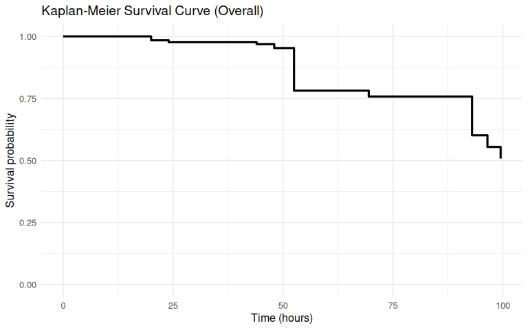
1.3.1.2 Families
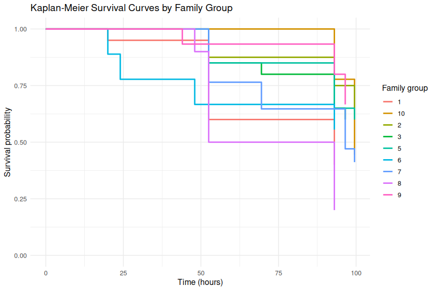
ggplot(km_family_df, aes(x = time, y = surv, color = family_group)) +
    geom_step(linewidth = 1.0) +
    labs(
        title = "Kaplan-Meier Survival Curves by Family Group",
        x = "Time (hours)",
        y = "Survival probability",
        color = "Family group"
    ) +
    ylim(0, 1) +
    theme_minimal(base_size = 12)