INTRO
This post presents results from resazurin assays conducted on families of Magallana gigas (Pacific oyster) in response to freshwater stress at room temperature (~21°C) over the course of 32hrs.
METHODS
Resazurin assays
M. gigas oysters from nine USDA families were placed individually in clear 12-well plates and submerged in 4 mL of resazurin working solution prepared with TAPWATER to induce a freshwater stress response. Plates were held at room temperature (~20°C) for the duration of the experiment (~32 h). At each designated timepoint, plates were transferred to a Synergy HTX (Agilent) plate reader and fluorescence was measured directly in the 12-well plates using the Gen5 software (Agilent).
Oyster measurements
Oyster area was measured using ImageJ. Oysters were photographed in their plates with a ruler for scale, and the area of each oyster was calculated using ImageJ “Measure Particles” tool.
Data analysis
Analysis was conducted in this R Markdown file:
The rendered markdown is below.
RESULTS
A significant effect of family on AUC-based metabolism was detected (one-way ANOVA: F(8, 90) = 3.28, p = 0.0025). Families 9b (mean AUC = 0.956 ± 0.076 SE) and 9 (0.871 ± 0.106) exhibited the highest metabolic activity, while families 7 (0.414 ± 0.042) and 6 (0.442 ± 0.031) showed the lowest. Tukey-adjusted pairwise comparisons identified significant AUC differences between families 7 and 9b (p = 0.0096) and families 6 and 9b (p = 0.0176).
Linear mixed-effects time-series modeling confirmed significant effects of time (F(9, 810) = 264.96, p < 0.001), family (F(8, 90) = 2.76, p = 0.009), and a time × family interaction (F(72, 810) = 2.29, p < 0.001). Family differences in metabolism were most pronounced at later timepoints (27.5–32 h), with families 6 and 7 showing significantly lower metabolism than families 9 and 9b during this period (Tukey-adjusted p < 0.05 for multiple comparisons).
1 Background
M. gigas oysters from nine USDA families were placed individually in clear 12-well plates and submerged in 4 mL of resazurin working solution prepared with tap water to induce a freshwater stress response. Plates were held at room temperature (~20°C) for the duration of the experiment (~32 h). At each designated timepoint, plates were transferred to a Synergy HTX (Agilent) plate reader and fluorescence was measured directly in the 12-well plates using the Gen5 software (Agilent).
See Resazurin/data/20260429-freshwater_stress/README.md for full experimental notes.
1.1 Expected inputs
| Path | Description |
|---|---|
Resazurin/data/20260429-freshwater_stress/plate-*-T*.txt |
Plate reader fluorescence exports (one file per plate per timepoint) |
Resazurin/data/20260429-freshwater_stress/layout.csv |
Well metadata: plate ID, well ID, blank flag, family groups, sample IDs, area measurements (mm², from ImageJ) |
1.2 Expected outputs
All outputs are written to Resazurin/outputs/01.00-resazurin-20260429-freshwater_stress/.
| File | Description |
|---|---|
figures/ |
All plots generated by this script |
auc_all_metrics.csv |
Per-individual AUC values for every active measurement metric |
auc_summary.csv |
Group-level AUC summary statistics (mean, SD, SE, median) |
metabolism.csv |
Full per-well per-timepoint metabolism data frame |
pairwise_stats.csv |
Tukey-adjusted pairwise comparisons from AUC linear models |
2 Setup
2.1 Knitr options
knitr::opts_chunk$set(
  echo = TRUE,         # Display code chunks
  eval = TRUE,        # Evaluate code chunks
  warning = FALSE,     # Hide warnings
  message = FALSE,     # Hide messages
  comment = "",         # Prevents appending '##' to beginning of lines in code output
  results = 'hold'     # Holds output so it's all printed together after code chunk
)
2.2 Load libraries
library(tidyverse)
library(pracma)       # trapz()
library(lme4)
library(lmerTest)
library(emmeans)
library(multcompView)
library(cowplot)
library(colorspace)   # qualitative_hcl() for large palettes
3 Helper Functions
normalize_well_id <- function(x) {
  x <- toupper(trimws(x))
  valid <- str_detect(x, "^[A-Z]+[0-9]+$")
  out <- rep(NA_character_, length(x))
  if (!any(valid)) return(out)
  m <- str_match(x[valid], "^([A-Z]+)([0-9]+)$")
  out[valid] <- paste0(m[, 2], as.integer(m[, 3]))
  out
}

parse_time_hr <- function(path) {
  hit <- str_match(basename(path),
                   "(?i)-T([0-9]+(?:\\.[0-9]+)?)\\.txt$")
  as.numeric(hit[, 2])
}

parse_plate_id <- function(path) {
  hit <- str_match(basename(path),
    "(?i)^plate-([A-Za-z0-9-]+)-T[0-9]+(?:\\.[0-9]+)?\\.txt$")
  id <- hit[, 2]
  ifelse(is.na(id), "unknown", id)
}

extract_results_block <- function(lines) {
  results_idx <- which(trimws(lines) == "Results")
  if (length(results_idx) == 0) stop("No Results section found")
  idx <- results_idx[1]
  header_tokens <- str_split(lines[idx + 1], "\\t")[[1]] |> trimws()
  col_ids <- header_tokens[
    header_tokens != "" & str_detect(header_tokens, "^[0-9]+$")]
  j <- idx + 2
  data_lines <- character()
  while (j <= length(lines)) {
    line <- lines[j]
    if (trimws(line) == "") break
    if (!str_detect(line, "^[A-Za-z]\\t")) break
    data_lines <- c(data_lines, line)
    j <- j + 1
  }
  list(col_ids = col_ids, data_lines = data_lines)
}

parse_plate_export <- function(path) {
  lines <- readLines(path, warn = FALSE)
  res <- extract_results_block(lines)

  map_dfr(res$data_lines, function(line) {
    tokens <- str_split(line, "\\t")[[1]] |> trimws()
    tokens <- tokens[tokens != ""]
    row_letter <- tokens[1]
    nums <- suppressWarnings(as.numeric(tokens[-1]))
    valid_idx <- which(!is.na(nums))
    if (length(valid_idx) == 0) return(tibble())
    vals <- nums[valid_idx]
    n <- min(length(vals), length(res$col_ids))
    tibble(
      row_id  = toupper(row_letter),
      col_id  = as.integer(res$col_ids[seq_len(n)]),
      well_id = normalize_well_id(
        paste0(toupper(row_letter), res$col_ids[seq_len(n)])),
      value   = vals[seq_len(n)]
    )
  }) %>%
    mutate(
      plate_id = str_to_lower(parse_plate_id(path)),
      time_hr  = parse_time_hr(path)
    )
}

trapezoid_auc <- function(time_hr, value) {
  ok <- is.finite(time_hr) & is.finite(value)
  t <- time_hr[ok]
  v <- value[ok]
  if (length(t) < 2) return(NA_real_)
  ord <- order(t)
  t <- t[ord]; v <- v[ord]
  sum(diff(t) * (head(v, -1) + tail(v, -1)) / 2)
}

# Shared helper: extract display unit string from a measurement column name.
# e.g. "area_mm2_measurement" -> "mm²", "weight_mg_measurement" -> "mg"
parse_meas_unit <- function(col_name) {
  unit_raw <- col_name |>
    str_remove("^metabolism_per_") |>
    str_remove("_measurement$") |>
    str_extract("[^_]+$")
  case_when(
    unit_raw == "mm2" ~ "mm²",
    unit_raw == "cm2" ~ "cm²",
    unit_raw == "mm3" ~ "mm³",
    unit_raw == "cm3" ~ "cm³",
    TRUE              ~ unit_raw
  )
}

# y-axis label for metabolism line plots: "fold change/mm²"
metabolism_y_label <- function(col_name) {
  paste0("Metabolism (fold change/", parse_meas_unit(col_name), ")")
}

# y-axis label for AUC box plots: "Metabolism (AUC; mm²)"
auc_y_label <- function(metric_name) {
  paste0("Metabolism (AUC; ", parse_meas_unit(metric_name), ")")
}
4 Load Data
4.1 Plate export files
proj_root <- rprojroot::find_rstudio_root_file()
data_dir  <- file.path(proj_root, "Resazurin", "data", "20260429-freshwater_stress")
out_dir   <- file.path(proj_root, "Resazurin", "outputs",
                        "01.00-resazurin-20260429-freshwater_stress")
fig_dir   <- file.path(out_dir, "figures")

dir.create(fig_dir, recursive = TRUE, showWarnings = FALSE)
dir.create(out_dir, recursive = TRUE, showWarnings = FALSE)

plate_files <- list.files(
  data_dir,
  pattern = "(?i)^plate-.*-T[0-9]+(?:\\.[0-9]+)?\\.txt$",
  full.names = TRUE
)

plate_raw <- map_dfr(plate_files, function(path) {
  tryCatch(parse_plate_export(path),
           error = function(e) {
             message("Parse error in ", basename(path), ": ", e$message)
             tibble()
           })
})

str(plate_raw)
tibble [1,080 × 6] (S3: tbl_df/tbl/data.frame)
$ row_id : chr [1:1080] "A" "A" "A" "A" ...
$ col_id : int [1:1080] 1 2 3 4 1 2 3 4 1 2 ...
$ well_id : chr [1:1080] "A1" "A2" "A3" "A4" ...
$ value : num [1:1080] 141 140 126 143 145 159 168 157 145 139 ...
$ plate_id: chr [1:1080] "a" "a" "a" "a" ...
$ time_hr : num [1:1080] 0 0 0 0 0 0 0 0 0 0 ...4.2 Plate consistency check
Checks that every plate has the same number of wells at every timepoint. The expected well count is the mode across all plate × timepoint reads. Any plate with at least one deviating read is flagged and dropped entirely before any further analysis — removing only the aberrant timepoint would break the fold-change baseline calculation.
well_counts <- plate_raw %>%
  group_by(plate_id, time_hr) %>%
  summarise(n_wells = n_distinct(well_id), .groups = "drop")

expected_n_wells <- as.integer(
  names(which.max(table(well_counts$n_wells)))
)

inconsistent_reads <- well_counts %>%
  filter(n_wells != expected_n_wells) %>%
  arrange(plate_id, time_hr)

inconsistent_plate_ids <- unique(inconsistent_reads$plate_id)

if (nrow(inconsistent_reads) > 0) {
  cat("**Plate consistency check FAILED.**",
      "Expected", expected_n_wells, "wells per plate-timepoint read.",
      length(inconsistent_plate_ids),
      "plate(s) have at least one deviating read and are excluded",
      "from all analyses:\n\n")
  cat(knitr::kable(
    inconsistent_reads,
    col.names = c("Plate", "Time (h)", "Wells read"),
    caption   = paste("Expected:", expected_n_wells, "wells per read")
  ), sep = "\n")
  cat("\n")
  plate_raw <- plate_raw %>%
    filter(!plate_id %in% inconsistent_plate_ids)
  message(length(inconsistent_plate_ids),
          " plate(s) removed from plate_raw: ",
          paste(inconsistent_plate_ids, collapse = ", "))
} else {
  cat("Plate consistency check passed: all",
      n_distinct(well_counts$plate_id), "plates have",
      expected_n_wells, "wells at every timepoint.\n")
}
Plate consistency check passed: all 9 plates have 12 wells at every timepoint.
4.3 Layout file
layout_path <- file.path(data_dir, "layout.csv")

layout_raw <- read_csv(layout_path,
                       col_types = cols(.default = "c"),
                       show_col_types = FALSE)

# Standardise column names to snake_case
names(layout_raw) <- names(layout_raw) |>
  str_to_lower() |>
  str_replace_all("[^a-z0-9]+", "_") |>
  str_replace_all("_+", "_") |>
  str_replace("_$", "")

# Normalise plate_id to match plate file ids (strip "plate-" prefix)
layout_clean <- layout_raw %>%
  mutate(
    plate_id = str_remove(str_to_lower(plate_id), "^plate-"),
    well_id  = normalize_well_id(plate_well),
    is_blank = if ("is_blank" %in% names(layout_raw))
      toupper(trimws(is_blank)) %in% c("TRUE", "T", "1", "YES", "Y")
    else
      FALSE
  )

found_exclude_col <- intersect(
  c("exclude_from_analysis", "exclude", "omit", "not_analyzed"),
  names(layout_clean)
)[1]
layout_clean <- layout_clean %>%
  mutate(
    exclude_from_analysis = if (!is.na(found_exclude_col))
      toupper(trimws(.data[[found_exclude_col]])) %in%
        c("TRUE", "T", "1", "YES", "Y")
    else
      FALSE
  )

# Identify measurement columns and group columns
measurement_cols <- names(layout_clean)[
  str_detect(names(layout_clean), "_measurement$")]
group_cols <- names(layout_clean)[
  str_detect(names(layout_clean), "_group$")]

# Cast measurement columns to numeric
layout_clean <- layout_clean %>%
  mutate(across(all_of(measurement_cols),
                ~ suppressWarnings(as.numeric(.x))))

# Determine which measurement columns actually contain finite data
active_meas_cols <- measurement_cols[
  sapply(measurement_cols, function(col)
    any(is.finite(layout_clean[[col]]), na.rm = TRUE))]

# Normalise group values to lowercase so they match colour scale definitions
layout_clean <- layout_clean %>%
  mutate(across(all_of(group_cols),
                ~ str_to_lower(trimws(as.character(.x)))))

message("Group columns: ", paste(group_cols, collapse = ", "))
message("Active measurement columns: ",
        paste(active_meas_cols, collapse = ", "))

str(layout_clean)
tibble [108 × 14] (S3: tbl_df/tbl/data.frame)
$ plate_id : chr [1:108] "a" "a" "a" "a" ...
$ plate_well : chr [1:108] "A01" "A02" "A03" "A04" ...
$ is_blank : logi [1:108] FALSE FALSE FALSE FALSE FALSE FALSE ...
$ family_id_group : chr [1:108] "6" "6" "6" "6" ...
$ sample_id_group : chr [1:108] "1" "2" "3" "4" ...
$ exclude_from_analysis: logi [1:108] FALSE FALSE FALSE FALSE FALSE FALSE ...
$ exclude_reason : chr [1:108] NA NA NA NA ...
$ weight_g_measurement : num [1:108] NA NA NA NA NA NA NA NA NA NA ...
$ width_mm_measurement : num [1:108] NA NA NA NA NA NA NA NA NA NA ...
$ length_mm_measurement: num [1:108] NA NA NA NA NA NA NA NA NA NA ...
$ treatment_group : chr [1:108] NA NA NA NA ...
$ area_mm2_measurement : num [1:108] 158 164 111 180 195 ...
$ imagej_id : chr [1:108] "2" "1" "3" "4" ...
$ well_id : chr [1:108] "A1" "A2" "A3" "A4" ...5 Merge Plate Data with Layout
dat <- plate_raw %>%
  left_join(
    layout_clean %>%
      select(plate_id, well_id, is_blank, exclude_from_analysis,
             any_of("exclude_reason"),
             all_of(group_cols), all_of(measurement_cols)),
    by = c("plate_id", "well_id")
  ) %>%
  mutate(
    is_blank = replace_na(is_blank, FALSE),
    exclude_from_analysis = replace_na(exclude_from_analysis, FALSE)
  )

str(dat)
tibble [1,080 × 16] (S3: tbl_df/tbl/data.frame)
$ row_id : chr [1:1080] "A" "A" "A" "A" ...
$ col_id : int [1:1080] 1 2 3 4 1 2 3 4 1 2 ...
$ well_id : chr [1:1080] "A1" "A2" "A3" "A4" ...
$ value : num [1:1080] 141 140 126 143 145 159 168 157 145 139 ...
$ plate_id : chr [1:1080] "a" "a" "a" "a" ...
$ time_hr : num [1:1080] 0 0 0 0 0 0 0 0 0 0 ...
$ is_blank : logi [1:1080] FALSE FALSE FALSE FALSE FALSE FALSE ...
$ exclude_from_analysis: logi [1:1080] FALSE FALSE FALSE FALSE FALSE FALSE ...
$ exclude_reason : chr [1:1080] NA NA NA NA ...
$ family_id_group : chr [1:1080] "6" "6" "6" "6" ...
$ sample_id_group : chr [1:1080] "1" "2" "3" "4" ...
$ treatment_group : chr [1:1080] NA NA NA NA ...
$ weight_g_measurement : num [1:1080] NA NA NA NA NA NA NA NA NA NA ...
$ width_mm_measurement : num [1:1080] NA NA NA NA NA NA NA NA NA NA ...
$ length_mm_measurement: num [1:1080] NA NA NA NA NA NA NA NA NA NA ...
$ area_mm2_measurement : num [1:1080] 158 164 111 180 195 ...6 Raw Fluorescence
6.1 Data frame
# Wells in the plate reader output that have no layout entry get all-NA group
# columns after the join. Keep only wells assigned to at least one group.
active_gc <- intersect(group_cols, names(dat))

raw_df <- dat %>%
  filter(
    !is_blank,
    if (length(active_gc) > 0)
      if_any(all_of(active_gc), ~ !is.na(.))
    else
      TRUE
  ) %>%
  mutate(
    trace_id = if_else(
      !is.na(sample_id_group) & trimws(as.character(sample_id_group)) != "",
      as.character(sample_id_group),
      paste(plate_id, well_id, sep = "_")
    )
  )

families   <- sort(unique(na.omit(raw_df$family_id_group)))
treatments <- sort(unique(na.omit(raw_df$treatment_group)))

n_fam <- length(families)
n_trt <- length(treatments)

# Palette strategy:
#   <= 7 groups : Okabe-Ito (gold standard for colorblind-safe figures).
#   >  7 groups : colorspace::qualitative_hcl("Dynamic") scales to any N
#                 using perceptually uniform HCL space — no colour collisions.
# Black (#000000) is excluded from both and reserved for blank wells.
okabe_ito_7 <- c(
  "#E69F00", "#56B4E9", "#009E73", "#F0E442",
  "#0072B2", "#D55E00", "#CC79A7"
)
make_palette <- function(n) {
  if (n == 0L) return(character(0))
  if (n <= length(okabe_ito_7)) return(okabe_ito_7[seq_len(n)])
  colorspace::qualitative_hcl(n, palette = "Dynamic")
}

all_colours   <- make_palette(n_fam + n_trt)
fam_colours   <- setNames(all_colours[seq_len(n_fam)], families)
trt_colours   <- setNames(all_colours[n_fam + seq_len(n_trt)], treatments)

lty_pool <- c("solid", "dashed", "dotted", "dotdash", "longdash")
trt_linetypes <- setNames(
  lty_pool[(seq_len(n_trt) - 1L) %% length(lty_pool) + 1L],
  treatments
)
plate_well_colours <- c(blank = "black", fam_colours)

has_trt <- n_trt > 0

str(raw_df)
tibble [990 × 17] (S3: tbl_df/tbl/data.frame)
$ row_id : chr [1:990] "A" "A" "A" "A" ...
$ col_id : int [1:990] 1 2 3 4 1 2 3 4 1 2 ...
$ well_id : chr [1:990] "A1" "A2" "A3" "A4" ...
$ value : num [1:990] 141 140 126 143 145 159 168 157 145 139 ...
$ plate_id : chr [1:990] "a" "a" "a" "a" ...
$ time_hr : num [1:990] 0 0 0 0 0 0 0 0 0 0 ...
$ is_blank : logi [1:990] FALSE FALSE FALSE FALSE FALSE FALSE ...
$ exclude_from_analysis: logi [1:990] FALSE FALSE FALSE FALSE FALSE FALSE ...
$ exclude_reason : chr [1:990] NA NA NA NA ...
$ family_id_group : chr [1:990] "6" "6" "6" "6" ...
$ sample_id_group : chr [1:990] "1" "2" "3" "4" ...
$ treatment_group : chr [1:990] NA NA NA NA ...
$ weight_g_measurement : num [1:990] NA NA NA NA NA NA NA NA NA NA ...
$ width_mm_measurement : num [1:990] NA NA NA NA NA NA NA NA NA NA ...
$ length_mm_measurement: num [1:990] NA NA NA NA NA NA NA NA NA NA ...
$ area_mm2_measurement : num [1:990] 158 164 111 180 195 ...
$ trace_id : chr [1:990] "1" "2" "3" "4" ...6.2 Raw fluorescence by plate (including blanks)
p_raw_plates <- dat %>%
  filter(is.finite(time_hr), is.finite(value)) %>%
  mutate(
    colour_group = if_else(is_blank, "blank",
                           coalesce(family_id_group, "sample")),
    trace_id     = paste(plate_id, well_id, sep = "_")
  ) %>%
  ggplot(aes(x = time_hr, y = value,
             group = trace_id, colour = colour_group)) +
  geom_line(alpha = 0.6) +
  geom_point(size = 1, alpha = 0.7) +
  facet_wrap(~ plate_id) +
  scale_colour_manual(
    values   = plate_well_colours,
    name     = "Group",
    breaks   = names(plate_well_colours),
    na.value = "grey80"
  ) +
  labs(x = "Time (h)", y = "Raw fluorescence (RFU)") +
  theme_classic(base_size = 12) +
  theme(strip.background = element_blank(),
        strip.text       = element_text(face = "bold"))

p_raw_plates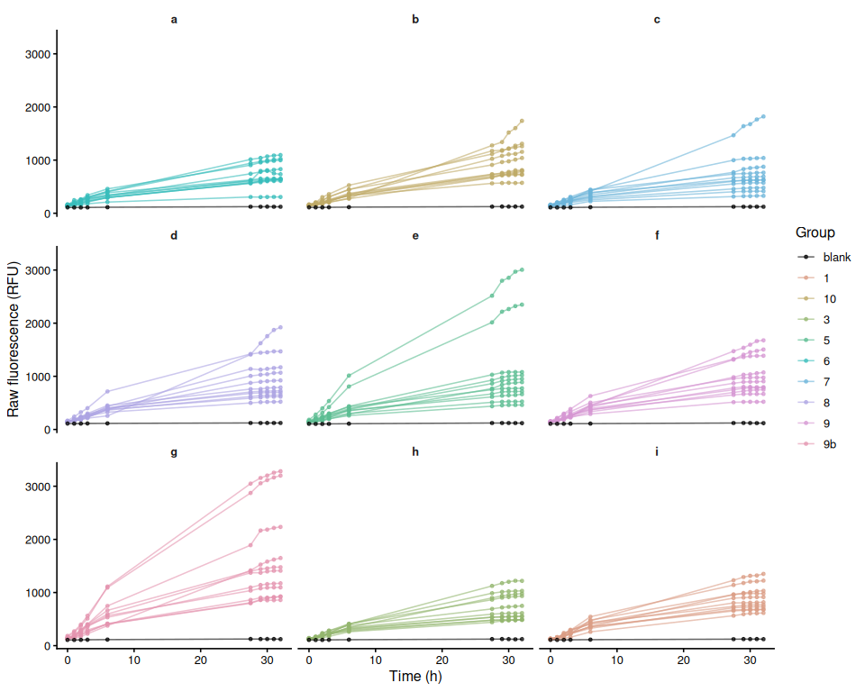
ggsave(file.path(fig_dir, "raw_fluor_by_plate.png"),
       p_raw_plates, width = 10, height = 8)
6.3 Mean raw fluorescence by family
raw_family_summary <- raw_df %>%
  filter(!is.na(family_id_group), !exclude_from_analysis) %>%
  group_by(family_id_group, treatment_group, time_hr) %>%
  summarise(
    mean_fluor = mean(value, na.rm = TRUE),
    se_fluor   = sd(value, na.rm = TRUE) /
      sqrt(sum(!is.na(value))),
    n          = sum(!is.na(value)),
    .groups    = "drop"
  ) %>%
  mutate(group_var = if (has_trt)
    paste(family_id_group, treatment_group, sep = ".")
  else
    family_id_group)

p_raw_mean <- ggplot(raw_family_summary,
    aes(x = time_hr, y = mean_fluor,
        colour = family_id_group,
        group = group_var)) +
  geom_ribbon(aes(ymin = mean_fluor - se_fluor,
                  ymax = mean_fluor + se_fluor,
                  fill = family_id_group),
              alpha = 0.15, colour = NA) +
  geom_line(
    mapping   = if (has_trt) aes(linetype = treatment_group) else NULL,
    linewidth = 1) +
  geom_point(size = 2) +
  scale_colour_manual(values = fam_colours, name = "Family") +
  scale_fill_manual(values = fam_colours, name = "Family") +
  labs(x = "Time (h)", y = "Mean raw fluorescence (RFU ± SE)") +
  theme_classic(base_size = 13) +
  if (has_trt) scale_linetype_manual(values = trt_linetypes, name = "Treatment") else NULL

p_raw_mean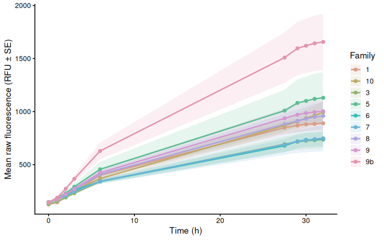
ggsave(file.path(fig_dir, "raw_mean_by_family.png"),
       p_raw_mean, width = 8, height = 5)
6.4 Individual raw fluorescence traces by family
p_raw_by_family <- raw_df %>%
  filter(!is.na(family_id_group)) %>%
  ggplot(aes(x = time_hr, y = value, group = trace_id,
             colour = .data[[if (has_trt) "treatment_group" else "family_id_group"]])) +
  geom_line(alpha = 0.6) +
  geom_point(size = 1.2, alpha = 0.7) +
  facet_wrap(~ family_id_group) +
  scale_colour_manual(
    values = if (has_trt) trt_colours else fam_colours,
    name   = if (has_trt) "Treatment" else "Family") +
  labs(x = "Time (h)", y = "Raw fluorescence (RFU)") +
  theme_classic(base_size = 12) +
  theme(strip.background = element_blank(),
        strip.text       = element_text(face = "bold"))

p_raw_by_family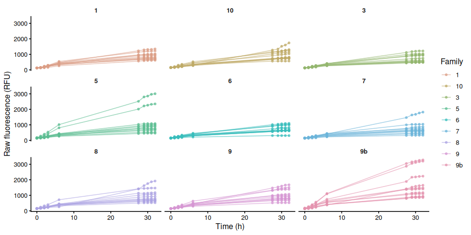
ggsave(file.path(fig_dir, "raw_individual_by_family.png"),
       p_raw_by_family, width = 10, height = 5)
6.5 Individual raw fluorescence traces by treatment
if (has_trt) {
  p_raw_by_treatment <- raw_df %>%
    ggplot(aes(x = time_hr, y = value,
               group = trace_id, colour = family_id_group)) +
    geom_line(alpha = 0.6) +
    geom_point(size = 1.2, alpha = 0.7) +
    facet_wrap(~ treatment_group) +
    scale_colour_manual(values = fam_colours, name = "Family") +
    labs(x = "Time (h)", y = "Raw fluorescence (RFU)") +
    theme_classic(base_size = 12) +
    theme(strip.background = element_blank(),
          strip.text       = element_text(face = "bold"))

  p_raw_by_treatment
  ggsave(file.path(fig_dir, "raw_individual_by_treatment.png"),
         p_raw_by_treatment, width = 10, height = 5)
}
6.6 Excluded samples
Wells flagged exclude_from_analysis = TRUE appear in the raw fluorescence plots above but are omitted from all analyses that follow.
excluded_wells <- dat %>%
  filter(!is_blank, exclude_from_analysis) %>%
  mutate(
    sample = if_else(
      !is.na(sample_id_group) & trimws(as.character(sample_id_group)) != "",
      as.character(sample_id_group),
      paste(plate_id, well_id, sep = "_")
    )
  ) %>%
  select(plate_id, well_id, sample, family_id_group, treatment_group,
         any_of("exclude_reason")) %>%
  distinct() %>%
  arrange(plate_id, well_id)

if (nrow(excluded_wells) > 0) {
  col_names <- c("Plate", "Well", "Sample", "Family", "Treatment")
  if ("exclude_reason" %in% names(excluded_wells))
    col_names <- c(col_names, "Reason")
  cat(knitr::kable(excluded_wells, col.names = col_names), sep = "\n")
} else {
  cat("No wells are excluded from analysis.\n")
}
No wells are excluded from analysis.
7 Blank Correction via Fold-Change Normalization
T0 is the earliest timepoint present in the dataset (not necessarily 0 hr). Sample fold-change is expressed relative to each individual’s T0 reading, resolved by sample_id_group when that column is populated — allowing the same animal to be tracked across plates — or by plate_id + well_id when no sample IDs exist (backward-compatible with single-plate, multi-timepoint designs). Blank fold-change is the per-plate mean blank RFU at each timepoint divided by the pooled mean blank RFU at T0. Subtracting blank fold-change from sample fold-change removes background fluorescence drift; all samples start at exactly 0 at T0 by construction.
7.1 Step 1 – Identify T0 and compute per-sample fold-change
# T0 = earliest timepoint present in the dataset
t0_time <- min(dat$time_hr[is.finite(dat$time_hr)], na.rm = TRUE)
message("T0 timepoint: ", t0_time, " hr")

# T0 reference value per individual.
# Resolved by sample_id_group (cross-plate tracking) when available;
# falls back to plate+well for layouts without explicit sample IDs.
t0_all <- dat %>%
  filter(time_hr == t0_time, !is_blank, is.finite(value)) %>%
  mutate(sample_key = if_else(
    !is.na(sample_id_group) & trimws(as.character(sample_id_group)) != "",
    as.character(sample_id_group),
    paste(plate_id, well_id, sep = "_")
  )) %>%
  group_by(sample_key) %>%
  summarise(value_t0 = mean(value, na.rm = TRUE), .groups = "drop")

dat_fc <- dat %>%
  mutate(sample_key = if_else(
    !is_blank &
      !is.na(sample_id_group) & trimws(as.character(sample_id_group)) != "",
    as.character(sample_id_group),
    paste(plate_id, well_id, sep = "_")
  )) %>%
  left_join(t0_all, by = "sample_key") %>%
  mutate(fold_change = if_else(
    !is_blank & is.finite(value_t0) & value_t0 > 0,
    value / value_t0,
    NA_real_
  ))

str(dat_fc)
tibble [1,080 × 19] (S3: tbl_df/tbl/data.frame)
$ row_id : chr [1:1080] "A" "A" "A" "A" ...
$ col_id : int [1:1080] 1 2 3 4 1 2 3 4 1 2 ...
$ well_id : chr [1:1080] "A1" "A2" "A3" "A4" ...
$ value : num [1:1080] 141 140 126 143 145 159 168 157 145 139 ...
$ plate_id : chr [1:1080] "a" "a" "a" "a" ...
$ time_hr : num [1:1080] 0 0 0 0 0 0 0 0 0 0 ...
$ is_blank : logi [1:1080] FALSE FALSE FALSE FALSE FALSE FALSE ...
$ exclude_from_analysis: logi [1:1080] FALSE FALSE FALSE FALSE FALSE FALSE ...
$ exclude_reason : chr [1:1080] NA NA NA NA ...
$ family_id_group : chr [1:1080] "6" "6" "6" "6" ...
$ sample_id_group : chr [1:1080] "1" "2" "3" "4" ...
$ treatment_group : chr [1:1080] NA NA NA NA ...
$ weight_g_measurement : num [1:1080] NA NA NA NA NA NA NA NA NA NA ...
$ width_mm_measurement : num [1:1080] NA NA NA NA NA NA NA NA NA NA ...
$ length_mm_measurement: num [1:1080] NA NA NA NA NA NA NA NA NA NA ...
$ area_mm2_measurement : num [1:1080] 158 164 111 180 195 ...
$ sample_key : chr [1:1080] "1" "2" "3" "4" ...
$ value_t0 : num [1:1080] 141 140 126 143 145 159 168 157 145 139 ...
$ fold_change : num [1:1080] 1 1 1 1 1 1 1 1 1 1 ...7.2 Step 2 – Blank fold-change reference per plate per timepoint
# Pooled mean blank RFU at T0 across all T0 plates
mean_blank_t0 <- dat %>%
  filter(is_blank, time_hr == t0_time, is.finite(value)) %>%
  pull(value) %>%
  mean(na.rm = TRUE)

if (!is.finite(mean_blank_t0))
  message("No blank readings found at T0 (", t0_time,
          " hr); blank correction will produce NA.")

# Per-plate per-timepoint mean blank expressed as fold-change relative to T0
blank_fc_ref <- dat %>%
  filter(is_blank, is.finite(value)) %>%
  group_by(plate_id, time_hr) %>%
  summarise(mean_blank_rfu = mean(value, na.rm = TRUE), .groups = "drop") %>%
  mutate(mean_blank_fc = mean_blank_rfu / mean_blank_t0)

str(blank_fc_ref)
tibble [90 × 4] (S3: tbl_df/tbl/data.frame)
$ plate_id : chr [1:90] "a" "a" "a" "a" ...
$ time_hr : num [1:90] 0 1 2 3 6 27.5 29 30 31 32 ...
$ mean_blank_rfu: num [1:90] 110 108 108 109 113 123 122 124 122 122 ...
$ mean_blank_fc : num [1:90] 1.011 0.993 0.993 1.002 1.039 ...7.3 Step 3 – Subtract blank fold-change from sample fold-change
samples <- dat_fc %>%
  filter(!is_blank, !exclude_from_analysis) %>%
  mutate(
    trace_id = if_else(
      !is.na(sample_id_group) & trimws(as.character(sample_id_group)) != "",
      as.character(sample_id_group),
      paste(plate_id, well_id, sep = "_")
    )
  ) %>%
  left_join(blank_fc_ref, by = c("plate_id", "time_hr")) %>%
  mutate(corrected_fc = fold_change - mean_blank_fc)

str(samples)
tibble [990 × 23] (S3: tbl_df/tbl/data.frame)
$ row_id : chr [1:990] "A" "A" "A" "A" ...
$ col_id : int [1:990] 1 2 3 4 1 2 3 4 1 2 ...
$ well_id : chr [1:990] "A1" "A2" "A3" "A4" ...
$ value : num [1:990] 141 140 126 143 145 159 168 157 145 139 ...
$ plate_id : chr [1:990] "a" "a" "a" "a" ...
$ time_hr : num [1:990] 0 0 0 0 0 0 0 0 0 0 ...
$ is_blank : logi [1:990] FALSE FALSE FALSE FALSE FALSE FALSE ...
$ exclude_from_analysis: logi [1:990] FALSE FALSE FALSE FALSE FALSE FALSE ...
$ exclude_reason : chr [1:990] NA NA NA NA ...
$ family_id_group : chr [1:990] "6" "6" "6" "6" ...
$ sample_id_group : chr [1:990] "1" "2" "3" "4" ...
$ treatment_group : chr [1:990] NA NA NA NA ...
$ weight_g_measurement : num [1:990] NA NA NA NA NA NA NA NA NA NA ...
$ width_mm_measurement : num [1:990] NA NA NA NA NA NA NA NA NA NA ...
$ length_mm_measurement: num [1:990] NA NA NA NA NA NA NA NA NA NA ...
$ area_mm2_measurement : num [1:990] 158 164 111 180 195 ...
$ sample_key : chr [1:990] "1" "2" "3" "4" ...
$ value_t0 : num [1:990] 141 140 126 143 145 159 168 157 145 139 ...
$ fold_change : num [1:990] 1 1 1 1 1 1 1 1 1 1 ...
$ trace_id : chr [1:990] "1" "2" "3" "4" ...
$ mean_blank_rfu : num [1:990] 110 110 110 110 110 110 110 110 110 110 ...
$ mean_blank_fc : num [1:990] 1.01 1.01 1.01 1.01 1.01 ...
$ corrected_fc : num [1:990] -0.0112 -0.0112 -0.0112 -0.0112 -0.0112 ...8 Blank-Corrected Fold-Change
8.1 Mean by family
bc_fc_summary <- samples %>%
  filter(!is.na(family_id_group), !exclude_from_analysis) %>%
  group_by(family_id_group, treatment_group, time_hr) %>%
  summarise(
    mean_val = mean(corrected_fc, na.rm = TRUE),
    se_val   = sd(corrected_fc, na.rm = TRUE) /
      sqrt(sum(!is.na(corrected_fc))),
    n        = sum(!is.na(corrected_fc)),
    .groups  = "drop"
  ) %>%
  mutate(group_var = if (has_trt)
    paste(family_id_group, treatment_group, sep = ".")
  else
    family_id_group)

p_bc_fc_mean <- ggplot(bc_fc_summary,
    aes(x = time_hr, y = mean_val,
        colour = family_id_group,
        group = group_var)) +
  geom_ribbon(aes(ymin = mean_val - se_val,
                  ymax = mean_val + se_val,
                  fill = family_id_group),
              alpha = 0.15, colour = NA) +
  geom_line(
    mapping   = if (has_trt) aes(linetype = treatment_group) else NULL,
    linewidth = 1) +
  geom_point(size = 2) +
  scale_colour_manual(values = fam_colours, name = "Family") +
  scale_fill_manual(values = fam_colours, name = "Family") +
  labs(x = "Time (h)",
       y = "Mean blank-corrected fold-change (± SE)") +
  theme_classic(base_size = 13) +
  if (has_trt) scale_linetype_manual(values = trt_linetypes, name = "Treatment") else NULL

p_bc_fc_mean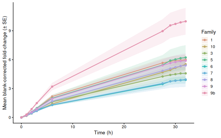
ggsave(file.path(fig_dir, "blank_corrected_fc_mean_by_family.png"),
       p_bc_fc_mean, width = 8, height = 5)
8.2 Individual traces by family
p_bc_fc_by_family <- samples %>%
  filter(!is.na(family_id_group)) %>%
  ggplot(aes(x = time_hr, y = corrected_fc, group = trace_id,
             colour = .data[[if (has_trt) "treatment_group" else "family_id_group"]])) +
  geom_line(alpha = 0.6) +
  geom_point(size = 1.2, alpha = 0.7) +
  facet_wrap(~ family_id_group) +
  scale_colour_manual(
    values = if (has_trt) trt_colours else fam_colours,
    name   = if (has_trt) "Treatment" else "Family") +
  labs(x = "Time (h)", y = "Blank-corrected fold-change") +
  theme_classic(base_size = 12) +
  theme(strip.background = element_blank(),
        strip.text       = element_text(face = "bold"))

p_bc_fc_by_family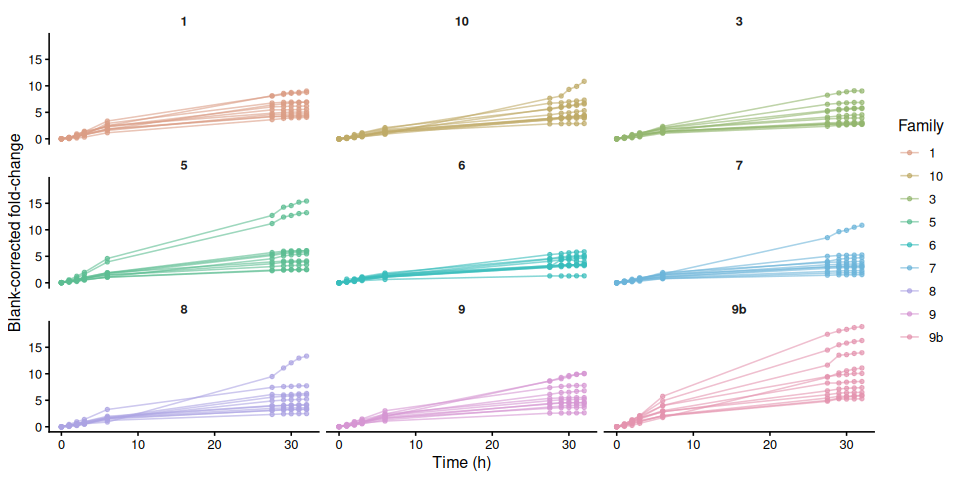
ggsave(file.path(fig_dir, "blank_corrected_fc_by_family.png"),
       p_bc_fc_by_family, width = 10, height = 5)
8.3 Individual blank-corrected fold-change traces by treatment
if (has_trt) {
p_bc_fc_by_treatment <- samples %>%
ggplot(aes(x = time_hr, y = corrected_fc,
group = trace_id, colour = family_id_group)) +
geom_line(alpha = 0.6) +
geom_point(size = 1.2, alpha = 0.7) +
facet_wrap(~ treatment_group) +
scale_colour_manual(values = fam_colours, name = "Family") +
labs(x = "Time (h)", y = "Blank-corrected fold-change") +
theme_classic(base_size = 12) +
theme(strip.background = element_blank(),
strip.text = element_text(face = "bold"))
p_bc_fc_by_treatment
ggsave(file.path(fig_dir, "blank_corrected_fc_by_treatment.png"),
p_bc_fc_by_treatment, width = 10, height = 5)
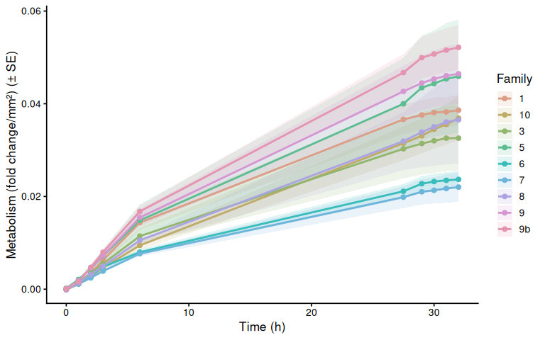
}9 Metabolism (Size-Normalised Fold-Change)
Blank-corrected fold-change divided by each active measurement column. This is “metabolism” as defined in Huffmyer et al.
if (length(active_meas_cols) == 0) {
  message("No active measurement columns: skipping metabolism calculation.")
  metabolism_df <- tibble()
} else {
  metabolism_df <- samples
  for (mc in active_meas_cols) {
    out_col <- paste0("metabolism_per_", mc)
    metabolism_df <- metabolism_df %>%
      mutate(!!out_col := if_else(
        is.finite(.data[[mc]]) & .data[[mc]] > 0 &
          is.finite(corrected_fc),
        corrected_fc / .data[[mc]],
        NA_real_
      ))
  }
}

str(metabolism_df)
tibble [990 × 24] (S3: tbl_df/tbl/data.frame)
$ row_id : chr [1:990] "A" "A" "A" "A" ...
$ col_id : int [1:990] 1 2 3 4 1 2 3 4 1 2 ...
$ well_id : chr [1:990] "A1" "A2" "A3" "A4" ...
$ value : num [1:990] 141 140 126 143 145 159 168 157 145 139 ...
$ plate_id : chr [1:990] "a" "a" "a" "a" ...
$ time_hr : num [1:990] 0 0 0 0 0 0 0 0 0 0 ...
$ is_blank : logi [1:990] FALSE FALSE FALSE FALSE FALSE FALSE ...
$ exclude_from_analysis : logi [1:990] FALSE FALSE FALSE FALSE FALSE FALSE ...
$ exclude_reason : chr [1:990] NA NA NA NA ...
$ family_id_group : chr [1:990] "6" "6" "6" "6" ...
$ sample_id_group : chr [1:990] "1" "2" "3" "4" ...
$ treatment_group : chr [1:990] NA NA NA NA ...
$ weight_g_measurement : num [1:990] NA NA NA NA NA NA NA NA NA NA ...
$ width_mm_measurement : num [1:990] NA NA NA NA NA NA NA NA NA NA ...
$ length_mm_measurement : num [1:990] NA NA NA NA NA NA NA NA NA NA ...
$ area_mm2_measurement : num [1:990] 158 164 111 180 195 ...
$ sample_key : chr [1:990] "1" "2" "3" "4" ...
$ value_t0 : num [1:990] 141 140 126 143 145 159 168 157 145 139 ...
$ fold_change : num [1:990] 1 1 1 1 1 1 1 1 1 1 ...
$ trace_id : chr [1:990] "1" "2" "3" "4" ...
$ mean_blank_rfu : num [1:990] 110 110 110 110 110 110 110 110 110 110 ...
$ mean_blank_fc : num [1:990] 1.01 1.01 1.01 1.01 1.01 ...
$ corrected_fc : num [1:990] -0.0112 -0.0112 -0.0112 -0.0112 -0.0112 ...
$ metabolism_per_area_mm2_measurement: num [1:990] -7.12e-05 -6.84e-05 -1.01e-04 -6.25e-05 -5.77e-05 ...9.1 Mean metabolism by family
if (nrow(metabolism_df) > 0) {

  metab_cols <- paste0("metabolism_per_", active_meas_cols)

  for (col in metab_cols) {
    if (!col %in% names(metabolism_df)) next
    mc_label <- str_remove(col, "^metabolism_per_")

    metab_summary <- metabolism_df %>%
      filter(!is.na(family_id_group), !exclude_from_analysis) %>%
      group_by(family_id_group, treatment_group, time_hr) %>%
      summarise(
        mean_val = mean(.data[[col]], na.rm = TRUE),
        se_val   = sd(.data[[col]], na.rm = TRUE) /
          sqrt(sum(!is.na(.data[[col]]))),
        .groups  = "drop"
      ) %>%
      mutate(group_var = if (has_trt)
        paste(family_id_group, treatment_group, sep = ".")
      else
        family_id_group)

    p_metab_mean <- ggplot(metab_summary,
        aes(x = time_hr, y = mean_val,
            colour = family_id_group,
            group = group_var)) +
      geom_ribbon(aes(ymin = mean_val - se_val,
                      ymax = mean_val + se_val,
                      fill = family_id_group),
                  alpha = 0.15, colour = NA) +
      geom_line(
        mapping   = if (has_trt) aes(linetype = treatment_group) else NULL,
        linewidth = 1) +
      geom_point(size = 2) +
      scale_colour_manual(values = fam_colours, name = "Family") +
      scale_fill_manual(values = fam_colours, name = "Family") +
      labs(x = "Time (h)",
           y = paste0(metabolism_y_label(col), " (± SE)")) +
      theme_classic(base_size = 13) +
      if (has_trt) scale_linetype_manual(values = trt_linetypes, name = "Treatment") else NULL

    print(p_metab_mean)
    ggsave(
      file.path(fig_dir,
                paste0("metabolism_mean_", mc_label, ".png")),
      p_metab_mean, width = 8, height = 5)
  }
}
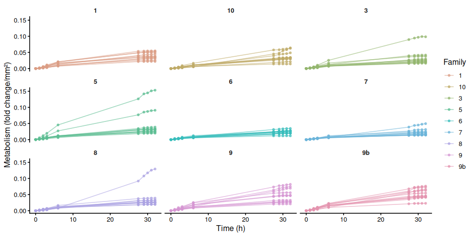
9.2 Individual metabolism traces by family
if (nrow(metabolism_df) > 0) {

  for (col in metab_cols) {
    if (!col %in% names(metabolism_df)) next
    mc_label <- str_remove(col, "^metabolism_per_")

    p_metab_by_family <- metabolism_df %>%
      filter(!is.na(family_id_group)) %>%
      ggplot(aes(x = time_hr, y = .data[[col]], group = trace_id,
                 colour = .data[[if (has_trt) "treatment_group" else "family_id_group"]])) +
      geom_line(alpha = 0.6) +
      geom_point(size = 1.2, alpha = 0.7) +
      facet_wrap(~ family_id_group) +
      scale_colour_manual(
        values = if (has_trt) trt_colours else fam_colours,
        name   = if (has_trt) "Treatment" else "Family") +
      labs(x = "Time (h)", y = metabolism_y_label(col)) +
      theme_classic(base_size = 12) +
      theme(strip.background = element_blank(),
            strip.text       = element_text(face = "bold"))

    print(p_metab_by_family)
    ggsave(
      file.path(fig_dir,
                paste0("metabolism_individual_", mc_label, "_by_family.png")),
      p_metab_by_family, width = 10, height = 5)

    if (has_trt) {
      p_metab_by_treatment <- ggplot(metabolism_df,
          aes(x = time_hr, y = .data[[col]],
              group = trace_id, colour = family_id_group)) +
        geom_line(alpha = 0.6) +
        geom_point(size = 1.2, alpha = 0.7) +
        facet_wrap(~ treatment_group) +
        scale_colour_manual(values = fam_colours, name = "Family") +
        labs(x = "Time (h)", y = metabolism_y_label(col)) +
        theme_classic(base_size = 12) +
        theme(strip.background = element_blank(),
              strip.text       = element_text(face = "bold"))

      print(p_metab_by_treatment)
      ggsave(
        file.path(fig_dir,
                  paste0("metabolism_individual_", mc_label, "_by_treatment.png")),
        p_metab_by_treatment, width = 10, height = 5)
    }
  }
}
10 Time-Series Statistical Analysis
Linear mixed effects models test the effect of experimental variables on metabolism over time. Individual (sample_id_group) is included as a random intercept to account for repeated measures across timepoints. Type III ANOVA with Satterthwaite’s approximation (lmerTest) assesses significance; post-hoc pairwise comparisons use estimated marginal means (emmeans, Tukey adjustment).
run_ts_stats <- function(df, value_col) {
  has_family    <- "family_id_group" %in% names(df) &&
    length(unique(na.omit(df$family_id_group))) > 1
  has_treatment <- "treatment_group" %in% names(df) &&
    length(unique(na.omit(df$treatment_group))) > 1

  if (!has_family && !has_treatment) return(NULL)

  df <- df %>%
    filter(is.finite(.data[[value_col]]), is.finite(time_hr)) %>%
    mutate(
      time_f     = factor(time_hr),
      individual = factor(trace_id)
    )

  if (nrow(df) == 0) return(NULL)

  if (has_family)    df <- df %>% mutate(family    = factor(family_id_group))
  if (has_treatment) df <- df %>% mutate(treatment = factor(treatment_group))

  if (has_family    && length(unique(na.omit(df$family)))    < 2) return(NULL)
  if (has_treatment && length(unique(na.omit(df$treatment))) < 2) return(NULL)

  fixed <- if (has_family && has_treatment) {
    paste0(value_col, " ~ time_f * family * treatment")
  } else if (has_family) {
    paste0(value_col, " ~ time_f * family")
  } else {
    paste0(value_col, " ~ time_f * treatment")
  }

  model <- lmer(
    as.formula(paste0(fixed, " + (1 | individual)")),
    data = df
  )

  anova_res <- anova(model, type = 3, ddf = "Satterthwaite")

  # Pairwise comparisons of group combinations at each timepoint
  emm_spec <- if (has_family && has_treatment) {
    ~ family * treatment | time_f
  } else if (has_family) {
    ~ family | time_f
  } else {
    ~ treatment | time_f
  }

  emm       <- emmeans(model, emm_spec)
  pairs_res <- as.data.frame(pairs(emm, adjust = "tukey"))

  # Main-effect marginal means (collapsed across time)
  emm_main <- if (has_family && has_treatment) {
    emmeans(model, ~ family * treatment)
  } else if (has_family) {
    emmeans(model, ~ family)
  } else {
    emmeans(model, ~ treatment)
  }

  pairs_main <- as.data.frame(pairs(emm_main, adjust = "tukey"))

  list(
    model         = model,
    anova         = anova_res,
    pairs_by_time = pairs_res,
    pairs_main    = pairs_main,
    has_family    = has_family,
    has_treatment = has_treatment
  )
}

ts_stats <- list()
if (nrow(metabolism_df) > 0) {
  for (mc in active_meas_cols) {
    col <- paste0("metabolism_per_", mc)
    if (col %in% names(metabolism_df))
      ts_stats[[col]] <- run_ts_stats(metabolism_df, col)
  }
}
10.1 Results
for (col in names(ts_stats)) {
  res <- ts_stats[[col]]
  if (is.null(res)) next

  cat("\n\n### Metric:", col, "\n\n")

  cat("**Type III ANOVA (Satterthwaite approximation):**\n\n")
  cat(knitr::kable(as.data.frame(res$anova), digits = 4, format = "pipe"), sep = "\n")
  cat("\n")

  cat("**Marginal means – main effects (collapsed across time):**\n\n")
  cat(knitr::kable(as.data.frame(res$pairs_main), digits = 4, format = "pipe"), sep = "\n")
  cat("\n")

  cat("**Pairwise comparisons by timepoint (Tukey):**\n\n")
  cat(knitr::kable(as.data.frame(res$pairs_by_time), digits = 4, format = "pipe"), sep = "\n")
  cat("\n")
}
10.1.1 Metric: metabolism_per_area_mm2_measurement
Type III ANOVA (Satterthwaite approximation):
| Sum Sq | Mean Sq | NumDF | DenDF | F value | Pr(>F) | |
|---|---|---|---|---|---|---|
| time_f | 0.2500 | 0.0278 | 9 | 810 | 264.9626 | 0.000 |
| family | 0.0023 | 0.0003 | 8 | 90 | 2.7567 | 0.009 |
| time_f:family | 0.0173 | 0.0002 | 72 | 810 | 2.2948 | 0.000 |
Marginal means – main effects (collapsed across time):
| contrast | estimate | SE | df | t.ratio | p.value |
|---|---|---|---|---|---|
| 1 - 10 | 0.0025 | 0.0046 | 90 | 0.5420 | 0.9998 |
| 1 - 3 | 0.0034 | 0.0046 | 90 | 0.7267 | 0.9983 |
| 1 - 5 | -0.0033 | 0.0046 | 90 | -0.7211 | 0.9984 |
| 1 - 6 | 0.0083 | 0.0046 | 90 | 1.7923 | 0.6870 |
| 1 - 7 | 0.0093 | 0.0046 | 90 | 2.0165 | 0.5362 |
| 1 - 8 | 0.0021 | 0.0046 | 90 | 0.4555 | 0.9999 |
| 1 - 9 | -0.0040 | 0.0046 | 90 | -0.8600 | 0.9944 |
| 1 - 9b | -0.0068 | 0.0046 | 90 | -1.4650 | 0.8685 |
| 10 - 3 | 0.0009 | 0.0046 | 90 | 0.1847 | 1.0000 |
| 10 - 5 | -0.0058 | 0.0046 | 90 | -1.2631 | 0.9392 |
| 10 - 6 | 0.0058 | 0.0046 | 90 | 1.2503 | 0.9426 |
| 10 - 7 | 0.0068 | 0.0046 | 90 | 1.4745 | 0.8643 |
| 10 - 8 | -0.0004 | 0.0046 | 90 | -0.0865 | 1.0000 |
| 10 - 9 | -0.0065 | 0.0046 | 90 | -1.4020 | 0.8942 |
| 10 - 9b | -0.0093 | 0.0046 | 90 | -2.0070 | 0.5427 |
| 3 - 5 | -0.0067 | 0.0046 | 90 | -1.4478 | 0.8758 |
| 3 - 6 | 0.0049 | 0.0046 | 90 | 1.0655 | 0.9776 |
| 3 - 7 | 0.0060 | 0.0046 | 90 | 1.2898 | 0.9318 |
| 3 - 8 | -0.0013 | 0.0046 | 90 | -0.2712 | 1.0000 |
| 3 - 9 | -0.0073 | 0.0046 | 90 | -1.5868 | 0.8094 |
| 3 - 9b | -0.0102 | 0.0046 | 90 | -2.1917 | 0.4199 |
| 5 - 6 | 0.0116 | 0.0046 | 90 | 2.5134 | 0.2397 |
| 5 - 7 | 0.0127 | 0.0046 | 90 | 2.7377 | 0.1497 |
| 5 - 8 | 0.0054 | 0.0046 | 90 | 1.1766 | 0.9594 |
| 5 - 9 | -0.0006 | 0.0046 | 90 | -0.1389 | 1.0000 |
| 5 - 9b | -0.0034 | 0.0046 | 90 | -0.7439 | 0.9980 |
| 6 - 7 | 0.0010 | 0.0046 | 90 | 0.2243 | 1.0000 |
| 6 - 8 | -0.0062 | 0.0046 | 90 | -1.3367 | 0.9174 |
| 6 - 9 | -0.0123 | 0.0046 | 90 | -2.6523 | 0.1804 |
| 6 - 9b | -0.0151 | 0.0046 | 90 | -3.2573 | 0.0402 |
| 7 - 8 | -0.0072 | 0.0046 | 90 | -1.5610 | 0.8229 |
| 7 - 9 | -0.0133 | 0.0046 | 90 | -2.8766 | 0.1084 |
| 7 - 9b | -0.0161 | 0.0046 | 90 | -3.4815 | 0.0210 |
| 8 - 9 | -0.0061 | 0.0046 | 90 | -1.3156 | 0.9241 |
| 8 - 9b | -0.0089 | 0.0046 | 90 | -1.9205 | 0.6016 |
| 9 - 9b | -0.0028 | 0.0046 | 90 | -0.6050 | 0.9995 |
Pairwise comparisons by timepoint (Tukey):
| contrast | time_f | estimate | SE | df | t.ratio | p.value |
|---|---|---|---|---|---|---|
| 1 - 10 | 0 | 0.0001 | 0.0062 | 272.2427 | 0.0202 | 1.0000 |
| 1 - 3 | 0 | -0.0001 | 0.0062 | 272.2427 | -0.0102 | 1.0000 |
| 1 - 5 | 0 | -0.0002 | 0.0062 | 272.2427 | -0.0316 | 1.0000 |
| 1 - 6 | 0 | 0.0001 | 0.0062 | 272.2427 | 0.0094 | 1.0000 |
| 1 - 7 | 0 | 0.0000 | 0.0062 | 272.2427 | -0.0002 | 1.0000 |
| 1 - 8 | 0 | 0.0001 | 0.0062 | 272.2427 | 0.0193 | 1.0000 |
| 1 - 9 | 0 | -0.0001 | 0.0062 | 272.2427 | -0.0231 | 1.0000 |
| 1 - 9b | 0 | -0.0001 | 0.0062 | 272.2427 | -0.0087 | 1.0000 |
| 10 - 3 | 0 | -0.0002 | 0.0062 | 272.2427 | -0.0304 | 1.0000 |
| 10 - 5 | 0 | -0.0003 | 0.0062 | 272.2427 | -0.0518 | 1.0000 |
| 10 - 6 | 0 | -0.0001 | 0.0062 | 272.2427 | -0.0108 | 1.0000 |
| 10 - 7 | 0 | -0.0001 | 0.0062 | 272.2427 | -0.0203 | 1.0000 |
| 10 - 8 | 0 | 0.0000 | 0.0062 | 272.2427 | -0.0009 | 1.0000 |
| 10 - 9 | 0 | -0.0003 | 0.0062 | 272.2427 | -0.0433 | 1.0000 |
| 10 - 9b | 0 | -0.0002 | 0.0062 | 272.2427 | -0.0288 | 1.0000 |
| 3 - 5 | 0 | -0.0001 | 0.0062 | 272.2427 | -0.0214 | 1.0000 |
| 3 - 6 | 0 | 0.0001 | 0.0062 | 272.2427 | 0.0196 | 1.0000 |
| 3 - 7 | 0 | 0.0001 | 0.0062 | 272.2427 | 0.0100 | 1.0000 |
| 3 - 8 | 0 | 0.0002 | 0.0062 | 272.2427 | 0.0294 | 1.0000 |
| 3 - 9 | 0 | -0.0001 | 0.0062 | 272.2427 | -0.0129 | 1.0000 |
| 3 - 9b | 0 | 0.0000 | 0.0062 | 272.2427 | 0.0015 | 1.0000 |
| 5 - 6 | 0 | 0.0003 | 0.0062 | 272.2427 | 0.0410 | 1.0000 |
| 5 - 7 | 0 | 0.0002 | 0.0062 | 272.2427 | 0.0314 | 1.0000 |
| 5 - 8 | 0 | 0.0003 | 0.0062 | 272.2427 | 0.0509 | 1.0000 |
| 5 - 9 | 0 | 0.0001 | 0.0062 | 272.2427 | 0.0085 | 1.0000 |
| 5 - 9b | 0 | 0.0001 | 0.0062 | 272.2427 | 0.0230 | 1.0000 |
| 6 - 7 | 0 | -0.0001 | 0.0062 | 272.2427 | -0.0096 | 1.0000 |
| 6 - 8 | 0 | 0.0001 | 0.0062 | 272.2427 | 0.0098 | 1.0000 |
| 6 - 9 | 0 | -0.0002 | 0.0062 | 272.2427 | -0.0325 | 1.0000 |
| 6 - 9b | 0 | -0.0001 | 0.0062 | 272.2427 | -0.0181 | 1.0000 |
| 7 - 8 | 0 | 0.0001 | 0.0062 | 272.2427 | 0.0194 | 1.0000 |
| 7 - 9 | 0 | -0.0001 | 0.0062 | 272.2427 | -0.0229 | 1.0000 |
| 7 - 9b | 0 | -0.0001 | 0.0062 | 272.2427 | -0.0085 | 1.0000 |
| 8 - 9 | 0 | -0.0003 | 0.0062 | 272.2427 | -0.0424 | 1.0000 |
| 8 - 9b | 0 | -0.0002 | 0.0062 | 272.2427 | -0.0279 | 1.0000 |
| 9 - 9b | 0 | 0.0001 | 0.0062 | 272.2427 | 0.0144 | 1.0000 |
| 1 - 10 | 1 | 0.0000 | 0.0062 | 272.2427 | 0.0021 | 1.0000 |
| 1 - 3 | 1 | -0.0004 | 0.0062 | 272.2427 | -0.0584 | 1.0000 |
| 1 - 5 | 1 | -0.0010 | 0.0062 | 272.2427 | -0.1539 | 1.0000 |
| 1 - 6 | 1 | -0.0004 | 0.0062 | 272.2427 | -0.0582 | 1.0000 |
| 1 - 7 | 1 | 0.0000 | 0.0062 | 272.2427 | 0.0040 | 1.0000 |
| 1 - 8 | 1 | -0.0002 | 0.0062 | 272.2427 | -0.0377 | 1.0000 |
| 1 - 9 | 1 | -0.0007 | 0.0062 | 272.2427 | -0.1146 | 1.0000 |
| 1 - 9b | 1 | -0.0005 | 0.0062 | 272.2427 | -0.0803 | 1.0000 |
| 10 - 3 | 1 | -0.0004 | 0.0062 | 272.2427 | -0.0604 | 1.0000 |
| 10 - 5 | 1 | -0.0010 | 0.0062 | 272.2427 | -0.1559 | 1.0000 |
| 10 - 6 | 1 | -0.0004 | 0.0062 | 272.2427 | -0.0602 | 1.0000 |
| 10 - 7 | 1 | 0.0000 | 0.0062 | 272.2427 | 0.0020 | 1.0000 |
| 10 - 8 | 1 | -0.0002 | 0.0062 | 272.2427 | -0.0397 | 1.0000 |
| 10 - 9 | 1 | -0.0007 | 0.0062 | 272.2427 | -0.1167 | 1.0000 |
| 10 - 9b | 1 | -0.0005 | 0.0062 | 272.2427 | -0.0824 | 1.0000 |
| 3 - 5 | 1 | -0.0006 | 0.0062 | 272.2427 | -0.0955 | 1.0000 |
| 3 - 6 | 1 | 0.0000 | 0.0062 | 272.2427 | 0.0002 | 1.0000 |
| 3 - 7 | 1 | 0.0004 | 0.0062 | 272.2427 | 0.0624 | 1.0000 |
| 3 - 8 | 1 | 0.0001 | 0.0062 | 272.2427 | 0.0207 | 1.0000 |
| 3 - 9 | 1 | -0.0003 | 0.0062 | 272.2427 | -0.0562 | 1.0000 |
| 3 - 9b | 1 | -0.0001 | 0.0062 | 272.2427 | -0.0219 | 1.0000 |
| 5 - 6 | 1 | 0.0006 | 0.0062 | 272.2427 | 0.0957 | 1.0000 |
| 5 - 7 | 1 | 0.0010 | 0.0062 | 272.2427 | 0.1579 | 1.0000 |
| 5 - 8 | 1 | 0.0007 | 0.0062 | 272.2427 | 0.1162 | 1.0000 |
| 5 - 9 | 1 | 0.0002 | 0.0062 | 272.2427 | 0.0393 | 1.0000 |
| 5 - 9b | 1 | 0.0005 | 0.0062 | 272.2427 | 0.0736 | 1.0000 |
| 6 - 7 | 1 | 0.0004 | 0.0062 | 272.2427 | 0.0622 | 1.0000 |
| 6 - 8 | 1 | 0.0001 | 0.0062 | 272.2427 | 0.0205 | 1.0000 |
| 6 - 9 | 1 | -0.0004 | 0.0062 | 272.2427 | -0.0564 | 1.0000 |
| 6 - 9b | 1 | -0.0001 | 0.0062 | 272.2427 | -0.0221 | 1.0000 |
| 7 - 8 | 1 | -0.0003 | 0.0062 | 272.2427 | -0.0417 | 1.0000 |
| 7 - 9 | 1 | -0.0007 | 0.0062 | 272.2427 | -0.1186 | 1.0000 |
| 7 - 9b | 1 | -0.0005 | 0.0062 | 272.2427 | -0.0843 | 1.0000 |
| 8 - 9 | 1 | -0.0005 | 0.0062 | 272.2427 | -0.0769 | 1.0000 |
| 8 - 9b | 1 | -0.0003 | 0.0062 | 272.2427 | -0.0426 | 1.0000 |
| 9 - 9b | 1 | 0.0002 | 0.0062 | 272.2427 | 0.0343 | 1.0000 |
| 1 - 10 | 2 | 0.0008 | 0.0062 | 272.2427 | 0.1221 | 1.0000 |
| 1 - 3 | 2 | 0.0001 | 0.0062 | 272.2427 | 0.0151 | 1.0000 |
| 1 - 5 | 2 | -0.0009 | 0.0062 | 272.2427 | -0.1455 | 1.0000 |
| 1 - 6 | 2 | 0.0006 | 0.0062 | 272.2427 | 0.0899 | 1.0000 |
| 1 - 7 | 2 | 0.0011 | 0.0062 | 272.2427 | 0.1705 | 1.0000 |
| 1 - 8 | 2 | 0.0004 | 0.0062 | 272.2427 | 0.0576 | 1.0000 |
| 1 - 9 | 2 | -0.0011 | 0.0062 | 272.2427 | -0.1711 | 1.0000 |
| 1 - 9b | 2 | -0.0012 | 0.0062 | 272.2427 | -0.1933 | 1.0000 |
| 10 - 3 | 2 | -0.0007 | 0.0062 | 272.2427 | -0.1070 | 1.0000 |
| 10 - 5 | 2 | -0.0017 | 0.0062 | 272.2427 | -0.2677 | 1.0000 |
| 10 - 6 | 2 | -0.0002 | 0.0062 | 272.2427 | -0.0322 | 1.0000 |
| 10 - 7 | 2 | 0.0003 | 0.0062 | 272.2427 | 0.0484 | 1.0000 |
| 10 - 8 | 2 | -0.0004 | 0.0062 | 272.2427 | -0.0645 | 1.0000 |
| 10 - 9 | 2 | -0.0018 | 0.0062 | 272.2427 | -0.2932 | 1.0000 |
| 10 - 9b | 2 | -0.0020 | 0.0062 | 272.2427 | -0.3155 | 1.0000 |
| 3 - 5 | 2 | -0.0010 | 0.0062 | 272.2427 | -0.1607 | 1.0000 |
| 3 - 6 | 2 | 0.0005 | 0.0062 | 272.2427 | 0.0748 | 1.0000 |
| 3 - 7 | 2 | 0.0010 | 0.0062 | 272.2427 | 0.1554 | 1.0000 |
| 3 - 8 | 2 | 0.0003 | 0.0062 | 272.2427 | 0.0425 | 1.0000 |
| 3 - 9 | 2 | -0.0012 | 0.0062 | 272.2427 | -0.1862 | 1.0000 |
| 3 - 9b | 2 | -0.0013 | 0.0062 | 272.2427 | -0.2085 | 1.0000 |
| 5 - 6 | 2 | 0.0015 | 0.0062 | 272.2427 | 0.2355 | 1.0000 |
| 5 - 7 | 2 | 0.0020 | 0.0062 | 272.2427 | 0.3161 | 1.0000 |
| 5 - 8 | 2 | 0.0013 | 0.0062 | 272.2427 | 0.2032 | 1.0000 |
| 5 - 9 | 2 | -0.0002 | 0.0062 | 272.2427 | -0.0255 | 1.0000 |
| 5 - 9b | 2 | -0.0003 | 0.0062 | 272.2427 | -0.0478 | 1.0000 |
| 6 - 7 | 2 | 0.0005 | 0.0062 | 272.2427 | 0.0806 | 1.0000 |
| 6 - 8 | 2 | -0.0002 | 0.0062 | 272.2427 | -0.0323 | 1.0000 |
| 6 - 9 | 2 | -0.0016 | 0.0062 | 272.2427 | -0.2610 | 1.0000 |
| 6 - 9b | 2 | -0.0018 | 0.0062 | 272.2427 | -0.2833 | 1.0000 |
| 7 - 8 | 2 | -0.0007 | 0.0062 | 272.2427 | -0.1129 | 1.0000 |
| 7 - 9 | 2 | -0.0021 | 0.0062 | 272.2427 | -0.3416 | 1.0000 |
| 7 - 9b | 2 | -0.0023 | 0.0062 | 272.2427 | -0.3639 | 1.0000 |
| 8 - 9 | 2 | -0.0014 | 0.0062 | 272.2427 | -0.2287 | 1.0000 |
| 8 - 9b | 2 | -0.0016 | 0.0062 | 272.2427 | -0.2510 | 1.0000 |
| 9 - 9b | 2 | -0.0001 | 0.0062 | 272.2427 | -0.0223 | 1.0000 |
| 1 - 10 | 3 | 0.0016 | 0.0062 | 272.2427 | 0.2625 | 1.0000 |
| 1 - 3 | 3 | 0.0008 | 0.0062 | 272.2427 | 0.1252 | 1.0000 |
| 1 - 5 | 3 | -0.0009 | 0.0062 | 272.2427 | -0.1445 | 1.0000 |
| 1 - 6 | 3 | 0.0014 | 0.0062 | 272.2427 | 0.2317 | 1.0000 |
| 1 - 7 | 3 | 0.0024 | 0.0062 | 272.2427 | 0.3817 | 1.0000 |
| 1 - 8 | 3 | 0.0013 | 0.0062 | 272.2427 | 0.2104 | 1.0000 |
| 1 - 9 | 3 | -0.0010 | 0.0062 | 272.2427 | -0.1582 | 1.0000 |
| 1 - 9b | 3 | -0.0017 | 0.0062 | 272.2427 | -0.2741 | 1.0000 |
| 10 - 3 | 3 | -0.0009 | 0.0062 | 272.2427 | -0.1373 | 1.0000 |
| 10 - 5 | 3 | -0.0025 | 0.0062 | 272.2427 | -0.4070 | 1.0000 |
| 10 - 6 | 3 | -0.0002 | 0.0062 | 272.2427 | -0.0307 | 1.0000 |
| 10 - 7 | 3 | 0.0007 | 0.0062 | 272.2427 | 0.1192 | 1.0000 |
| 10 - 8 | 3 | -0.0003 | 0.0062 | 272.2427 | -0.0520 | 1.0000 |
| 10 - 9 | 3 | -0.0026 | 0.0062 | 272.2427 | -0.4206 | 1.0000 |
| 10 - 9b | 3 | -0.0033 | 0.0062 | 272.2427 | -0.5366 | 0.9998 |
| 3 - 5 | 3 | -0.0017 | 0.0062 | 272.2427 | -0.2697 | 1.0000 |
| 3 - 6 | 3 | 0.0007 | 0.0062 | 272.2427 | 0.1065 | 1.0000 |
| 3 - 7 | 3 | 0.0016 | 0.0062 | 272.2427 | 0.2565 | 1.0000 |
| 3 - 8 | 3 | 0.0005 | 0.0062 | 272.2427 | 0.0853 | 1.0000 |
| 3 - 9 | 3 | -0.0018 | 0.0062 | 272.2427 | -0.2833 | 1.0000 |
| 3 - 9b | 3 | -0.0025 | 0.0062 | 272.2427 | -0.3993 | 1.0000 |
| 5 - 6 | 3 | 0.0023 | 0.0062 | 272.2427 | 0.3763 | 1.0000 |
| 5 - 7 | 3 | 0.0033 | 0.0062 | 272.2427 | 0.5262 | 0.9998 |
| 5 - 8 | 3 | 0.0022 | 0.0062 | 272.2427 | 0.3550 | 1.0000 |
| 5 - 9 | 3 | -0.0001 | 0.0062 | 272.2427 | -0.0136 | 1.0000 |
| 5 - 9b | 3 | -0.0008 | 0.0062 | 272.2427 | -0.1296 | 1.0000 |
| 6 - 7 | 3 | 0.0009 | 0.0062 | 272.2427 | 0.1499 | 1.0000 |
| 6 - 8 | 3 | -0.0001 | 0.0062 | 272.2427 | -0.0213 | 1.0000 |
| 6 - 9 | 3 | -0.0024 | 0.0062 | 272.2427 | -0.3899 | 1.0000 |
| 6 - 9b | 3 | -0.0031 | 0.0062 | 272.2427 | -0.5059 | 0.9999 |
| 7 - 8 | 3 | -0.0011 | 0.0062 | 272.2427 | -0.1712 | 1.0000 |
| 7 - 9 | 3 | -0.0034 | 0.0062 | 272.2427 | -0.5398 | 0.9998 |
| 7 - 9b | 3 | -0.0041 | 0.0062 | 272.2427 | -0.6558 | 0.9992 |
| 8 - 9 | 3 | -0.0023 | 0.0062 | 272.2427 | -0.3686 | 1.0000 |
| 8 - 9b | 3 | -0.0030 | 0.0062 | 272.2427 | -0.4846 | 0.9999 |
| 9 - 9b | 3 | -0.0007 | 0.0062 | 272.2427 | -0.1160 | 1.0000 |
| 1 - 10 | 6 | 0.0049 | 0.0062 | 272.2427 | 0.7906 | 0.9971 |
| 1 - 3 | 6 | 0.0029 | 0.0062 | 272.2427 | 0.4687 | 0.9999 |
| 1 - 5 | 6 | -0.0005 | 0.0062 | 272.2427 | -0.0768 | 1.0000 |
| 1 - 6 | 6 | 0.0064 | 0.0062 | 272.2427 | 1.0265 | 0.9831 |
| 1 - 7 | 6 | 0.0067 | 0.0062 | 272.2427 | 1.0779 | 0.9770 |
| 1 - 8 | 6 | 0.0038 | 0.0062 | 272.2427 | 0.6144 | 0.9995 |
| 1 - 9 | 6 | -0.0011 | 0.0062 | 272.2427 | -0.1753 | 1.0000 |
| 1 - 9b | 6 | -0.0024 | 0.0062 | 272.2427 | -0.3884 | 1.0000 |
| 10 - 3 | 6 | -0.0020 | 0.0062 | 272.2427 | -0.3219 | 1.0000 |
| 10 - 5 | 6 | -0.0054 | 0.0062 | 272.2427 | -0.8674 | 0.9944 |
| 10 - 6 | 6 | 0.0015 | 0.0062 | 272.2427 | 0.2359 | 1.0000 |
| 10 - 7 | 6 | 0.0018 | 0.0062 | 272.2427 | 0.2873 | 1.0000 |
| 10 - 8 | 6 | -0.0011 | 0.0062 | 272.2427 | -0.1762 | 1.0000 |
| 10 - 9 | 6 | -0.0060 | 0.0062 | 272.2427 | -0.9659 | 0.9886 |
| 10 - 9b | 6 | -0.0073 | 0.0062 | 272.2427 | -1.1790 | 0.9603 |
| 3 - 5 | 6 | -0.0034 | 0.0062 | 272.2427 | -0.5455 | 0.9998 |
| 3 - 6 | 6 | 0.0035 | 0.0062 | 272.2427 | 0.5578 | 0.9998 |
| 3 - 7 | 6 | 0.0038 | 0.0062 | 272.2427 | 0.6092 | 0.9996 |
| 3 - 8 | 6 | 0.0009 | 0.0062 | 272.2427 | 0.1456 | 1.0000 |
| 3 - 9 | 6 | -0.0040 | 0.0062 | 272.2427 | -0.6440 | 0.9993 |
| 3 - 9b | 6 | -0.0053 | 0.0062 | 272.2427 | -0.8571 | 0.9949 |
| 5 - 6 | 6 | 0.0069 | 0.0062 | 272.2427 | 1.1033 | 0.9734 |
| 5 - 7 | 6 | 0.0072 | 0.0062 | 272.2427 | 1.1546 | 0.9650 |
| 5 - 8 | 6 | 0.0043 | 0.0062 | 272.2427 | 0.6911 | 0.9989 |
| 5 - 9 | 6 | -0.0006 | 0.0062 | 272.2427 | -0.0986 | 1.0000 |
| 5 - 9b | 6 | -0.0019 | 0.0062 | 272.2427 | -0.3116 | 1.0000 |
| 6 - 7 | 6 | 0.0003 | 0.0062 | 272.2427 | 0.0514 | 1.0000 |
| 6 - 8 | 6 | -0.0026 | 0.0062 | 272.2427 | -0.4121 | 1.0000 |
| 6 - 9 | 6 | -0.0075 | 0.0062 | 272.2427 | -1.2018 | 0.9556 |
| 6 - 9b | 6 | -0.0088 | 0.0062 | 272.2427 | -1.4149 | 0.8914 |
| 7 - 8 | 6 | -0.0029 | 0.0062 | 272.2427 | -0.4635 | 0.9999 |
| 7 - 9 | 6 | -0.0078 | 0.0062 | 272.2427 | -1.2532 | 0.9436 |
| 7 - 9b | 6 | -0.0091 | 0.0062 | 272.2427 | -1.4662 | 0.8701 |
| 8 - 9 | 6 | -0.0049 | 0.0062 | 272.2427 | -0.7897 | 0.9971 |
| 8 - 9b | 6 | -0.0062 | 0.0062 | 272.2427 | -1.0027 | 0.9854 |
| 9 - 9b | 6 | -0.0013 | 0.0062 | 272.2427 | -0.2130 | 1.0000 |
| 1 - 10 | 27.5 | 0.0051 | 0.0062 | 272.2427 | 0.8258 | 0.9960 |
| 1 - 3 | 27.5 | 0.0063 | 0.0062 | 272.2427 | 1.0214 | 0.9836 |
| 1 - 5 | 27.5 | -0.0034 | 0.0062 | 272.2427 | -0.5419 | 0.9998 |
| 1 - 6 | 27.5 | 0.0155 | 0.0062 | 272.2427 | 2.4960 | 0.2385 |
| 1 - 7 | 27.5 | 0.0168 | 0.0062 | 272.2427 | 2.6991 | 0.1530 |
| 1 - 8 | 27.5 | 0.0047 | 0.0062 | 272.2427 | 0.7572 | 0.9978 |
| 1 - 9 | 27.5 | -0.0060 | 0.0062 | 272.2427 | -0.9720 | 0.9881 |
| 1 - 9b | 27.5 | -0.0101 | 0.0062 | 272.2427 | -1.6241 | 0.7909 |
| 10 - 3 | 27.5 | 0.0012 | 0.0062 | 272.2427 | 0.1956 | 1.0000 |
| 10 - 5 | 27.5 | -0.0085 | 0.0062 | 272.2427 | -1.3677 | 0.9090 |
| 10 - 6 | 27.5 | 0.0104 | 0.0062 | 272.2427 | 1.6702 | 0.7641 |
| 10 - 7 | 27.5 | 0.0116 | 0.0062 | 272.2427 | 1.8733 | 0.6328 |
| 10 - 8 | 27.5 | -0.0004 | 0.0062 | 272.2427 | -0.0686 | 1.0000 |
| 10 - 9 | 27.5 | -0.0112 | 0.0062 | 272.2427 | -1.7978 | 0.6837 |
| 10 - 9b | 27.5 | -0.0152 | 0.0062 | 272.2427 | -2.4499 | 0.2616 |
| 3 - 5 | 27.5 | -0.0097 | 0.0062 | 272.2427 | -1.5632 | 0.8238 |
| 3 - 6 | 27.5 | 0.0092 | 0.0062 | 272.2427 | 1.4747 | 0.8664 |
| 3 - 7 | 27.5 | 0.0104 | 0.0062 | 272.2427 | 1.6777 | 0.7597 |
| 3 - 8 | 27.5 | -0.0016 | 0.0062 | 272.2427 | -0.2641 | 1.0000 |
| 3 - 9 | 27.5 | -0.0124 | 0.0062 | 272.2427 | -1.9933 | 0.5494 |
| 3 - 9b | 27.5 | -0.0164 | 0.0062 | 272.2427 | -2.6455 | 0.1730 |
| 5 - 6 | 27.5 | 0.0189 | 0.0062 | 272.2427 | 3.0379 | 0.0643 |
| 5 - 7 | 27.5 | 0.0201 | 0.0062 | 272.2427 | 3.2409 | 0.0357 |
| 5 - 8 | 27.5 | 0.0081 | 0.0062 | 272.2427 | 1.2991 | 0.9310 |
| 5 - 9 | 27.5 | -0.0027 | 0.0062 | 272.2427 | -0.4301 | 1.0000 |
| 5 - 9b | 27.5 | -0.0067 | 0.0062 | 272.2427 | -1.0823 | 0.9764 |
| 6 - 7 | 27.5 | 0.0013 | 0.0062 | 272.2427 | 0.2030 | 1.0000 |
| 6 - 8 | 27.5 | -0.0108 | 0.0062 | 272.2427 | -1.7388 | 0.7219 |
| 6 - 9 | 27.5 | -0.0215 | 0.0062 | 272.2427 | -3.4680 | 0.0174 |
| 6 - 9b | 27.5 | -0.0256 | 0.0062 | 272.2427 | -4.1202 | 0.0016 |
| 7 - 8 | 27.5 | -0.0121 | 0.0062 | 272.2427 | -1.9418 | 0.5853 |
| 7 - 9 | 27.5 | -0.0228 | 0.0062 | 272.2427 | -3.6710 | 0.0087 |
| 7 - 9b | 27.5 | -0.0269 | 0.0062 | 272.2427 | -4.3232 | 0.0007 |
| 8 - 9 | 27.5 | -0.0107 | 0.0062 | 272.2427 | -1.7292 | 0.7280 |
| 8 - 9b | 27.5 | -0.0148 | 0.0062 | 272.2427 | -2.3814 | 0.2985 |
| 9 - 9b | 27.5 | -0.0041 | 0.0062 | 272.2427 | -0.6522 | 0.9993 |
| 1 - 10 | 29 | 0.0045 | 0.0062 | 272.2427 | 0.7207 | 0.9985 |
| 1 - 3 | 29 | 0.0061 | 0.0062 | 272.2427 | 0.9897 | 0.9866 |
| 1 - 5 | 29 | -0.0059 | 0.0062 | 272.2427 | -0.9506 | 0.9897 |
| 1 - 6 | 29 | 0.0148 | 0.0062 | 272.2427 | 2.3854 | 0.2962 |
| 1 - 7 | 29 | 0.0166 | 0.0062 | 272.2427 | 2.6658 | 0.1652 |
| 1 - 8 | 29 | 0.0037 | 0.0062 | 272.2427 | 0.5939 | 0.9996 |
| 1 - 9 | 29 | -0.0069 | 0.0062 | 272.2427 | -1.1108 | 0.9723 |
| 1 - 9b | 29 | -0.0124 | 0.0062 | 272.2427 | -1.9920 | 0.5503 |
| 10 - 3 | 29 | 0.0017 | 0.0062 | 272.2427 | 0.2690 | 1.0000 |
| 10 - 5 | 29 | -0.0104 | 0.0062 | 272.2427 | -1.6713 | 0.7635 |
| 10 - 6 | 29 | 0.0103 | 0.0062 | 272.2427 | 1.6647 | 0.7674 |
| 10 - 7 | 29 | 0.0121 | 0.0062 | 272.2427 | 1.9451 | 0.5830 |
| 10 - 8 | 29 | -0.0008 | 0.0062 | 272.2427 | -0.1268 | 1.0000 |
| 10 - 9 | 29 | -0.0114 | 0.0062 | 272.2427 | -1.8315 | 0.6611 |
| 10 - 9b | 29 | -0.0169 | 0.0062 | 272.2427 | -2.7127 | 0.1482 |
| 3 - 5 | 29 | -0.0121 | 0.0062 | 272.2427 | -1.9402 | 0.5864 |
| 3 - 6 | 29 | 0.0087 | 0.0062 | 272.2427 | 1.3957 | 0.8988 |
| 3 - 7 | 29 | 0.0104 | 0.0062 | 272.2427 | 1.6761 | 0.7606 |
| 3 - 8 | 29 | -0.0025 | 0.0062 | 272.2427 | -0.3958 | 1.0000 |
| 3 - 9 | 29 | -0.0131 | 0.0062 | 272.2427 | -2.1005 | 0.4752 |
| 3 - 9b | 29 | -0.0185 | 0.0062 | 272.2427 | -2.9817 | 0.0751 |
| 5 - 6 | 29 | 0.0207 | 0.0062 | 272.2427 | 3.3360 | 0.0266 |
| 5 - 7 | 29 | 0.0225 | 0.0062 | 272.2427 | 3.6164 | 0.0106 |
| 5 - 8 | 29 | 0.0096 | 0.0062 | 272.2427 | 1.5445 | 0.8334 |
| 5 - 9 | 29 | -0.0010 | 0.0062 | 272.2427 | -0.1603 | 1.0000 |
| 5 - 9b | 29 | -0.0065 | 0.0062 | 272.2427 | -1.0414 | 0.9814 |
| 6 - 7 | 29 | 0.0017 | 0.0062 | 272.2427 | 0.2804 | 1.0000 |
| 6 - 8 | 29 | -0.0111 | 0.0062 | 272.2427 | -1.7915 | 0.6878 |
| 6 - 9 | 29 | -0.0217 | 0.0062 | 272.2427 | -3.4962 | 0.0159 |
| 6 - 9b | 29 | -0.0272 | 0.0062 | 272.2427 | -4.3774 | 0.0006 |
| 7 - 8 | 29 | -0.0129 | 0.0062 | 272.2427 | -2.0719 | 0.4948 |
| 7 - 9 | 29 | -0.0235 | 0.0062 | 272.2427 | -3.7766 | 0.0060 |
| 7 - 9b | 29 | -0.0289 | 0.0062 | 272.2427 | -4.6578 | 0.0002 |
| 8 - 9 | 29 | -0.0106 | 0.0062 | 272.2427 | -1.7047 | 0.7433 |
| 8 - 9b | 29 | -0.0161 | 0.0062 | 272.2427 | -2.5859 | 0.1974 |
| 9 - 9b | 29 | -0.0055 | 0.0062 | 272.2427 | -0.8812 | 0.9938 |
| 1 - 10 | 30 | 0.0036 | 0.0062 | 272.2427 | 0.5827 | 0.9997 |
| 1 - 3 | 30 | 0.0061 | 0.0062 | 272.2427 | 0.9822 | 0.9872 |
| 1 - 5 | 30 | -0.0062 | 0.0062 | 272.2427 | -1.0042 | 0.9853 |
| 1 - 6 | 30 | 0.0149 | 0.0062 | 272.2427 | 2.3984 | 0.2890 |
| 1 - 7 | 30 | 0.0168 | 0.0062 | 272.2427 | 2.7021 | 0.1520 |
| 1 - 8 | 30 | 0.0031 | 0.0062 | 272.2427 | 0.4982 | 0.9999 |
| 1 - 9 | 30 | -0.0072 | 0.0062 | 272.2427 | -1.1633 | 0.9634 |
| 1 - 9b | 30 | -0.0126 | 0.0062 | 272.2427 | -2.0320 | 0.5224 |
| 10 - 3 | 30 | 0.0025 | 0.0062 | 272.2427 | 0.3994 | 1.0000 |
| 10 - 5 | 30 | -0.0099 | 0.0062 | 272.2427 | -1.5869 | 0.8113 |
| 10 - 6 | 30 | 0.0113 | 0.0062 | 272.2427 | 1.8157 | 0.6718 |
| 10 - 7 | 30 | 0.0132 | 0.0062 | 272.2427 | 2.1194 | 0.4623 |
| 10 - 8 | 30 | -0.0005 | 0.0062 | 272.2427 | -0.0845 | 1.0000 |
| 10 - 9 | 30 | -0.0108 | 0.0062 | 272.2427 | -1.7460 | 0.7174 |
| 10 - 9b | 30 | -0.0162 | 0.0062 | 272.2427 | -2.6147 | 0.1853 |
| 3 - 5 | 30 | -0.0123 | 0.0062 | 272.2427 | -1.9863 | 0.5543 |
| 3 - 6 | 30 | 0.0088 | 0.0062 | 272.2427 | 1.4162 | 0.8909 |
| 3 - 7 | 30 | 0.0107 | 0.0062 | 272.2427 | 1.7199 | 0.7338 |
| 3 - 8 | 30 | -0.0030 | 0.0062 | 272.2427 | -0.4839 | 0.9999 |
| 3 - 9 | 30 | -0.0133 | 0.0062 | 272.2427 | -2.1454 | 0.4447 |
| 3 - 9b | 30 | -0.0187 | 0.0062 | 272.2427 | -3.0141 | 0.0687 |
| 5 - 6 | 30 | 0.0211 | 0.0062 | 272.2427 | 3.4026 | 0.0216 |
| 5 - 7 | 30 | 0.0230 | 0.0062 | 272.2427 | 3.7062 | 0.0077 |
| 5 - 8 | 30 | 0.0093 | 0.0062 | 272.2427 | 1.5024 | 0.8538 |
| 5 - 9 | 30 | -0.0010 | 0.0062 | 272.2427 | -0.1591 | 1.0000 |
| 5 - 9b | 30 | -0.0064 | 0.0062 | 272.2427 | -1.0278 | 0.9829 |
| 6 - 7 | 30 | 0.0019 | 0.0062 | 272.2427 | 0.3037 | 1.0000 |
| 6 - 8 | 30 | -0.0118 | 0.0062 | 272.2427 | -1.9002 | 0.6142 |
| 6 - 9 | 30 | -0.0221 | 0.0062 | 272.2427 | -3.5617 | 0.0127 |
| 6 - 9b | 30 | -0.0275 | 0.0062 | 272.2427 | -4.4304 | 0.0005 |
| 7 - 8 | 30 | -0.0137 | 0.0062 | 272.2427 | -2.2038 | 0.4061 |
| 7 - 9 | 30 | -0.0240 | 0.0062 | 272.2427 | -3.8654 | 0.0043 |
| 7 - 9b | 30 | -0.0294 | 0.0062 | 272.2427 | -4.7340 | 0.0001 |
| 8 - 9 | 30 | -0.0103 | 0.0062 | 272.2427 | -1.6615 | 0.7693 |
| 8 - 9b | 30 | -0.0157 | 0.0062 | 272.2427 | -2.5302 | 0.2223 |
| 9 - 9b | 30 | -0.0054 | 0.0062 | 272.2427 | -0.8687 | 0.9944 |
| 1 - 10 | 31 | 0.0027 | 0.0062 | 272.2427 | 0.4337 | 1.0000 |
| 1 - 3 | 31 | 0.0057 | 0.0062 | 272.2427 | 0.9113 | 0.9922 |
| 1 - 5 | 31 | -0.0071 | 0.0062 | 272.2427 | -1.1486 | 0.9660 |
| 1 - 6 | 31 | 0.0148 | 0.0062 | 272.2427 | 2.3755 | 0.3018 |
| 1 - 7 | 31 | 0.0165 | 0.0062 | 272.2427 | 2.6590 | 0.1678 |
| 1 - 8 | 31 | 0.0022 | 0.0062 | 272.2427 | 0.3492 | 1.0000 |
| 1 - 9 | 31 | -0.0078 | 0.0062 | 272.2427 | -1.2586 | 0.9422 |
| 1 - 9b | 31 | -0.0133 | 0.0062 | 272.2427 | -2.1468 | 0.4438 |
| 10 - 3 | 31 | 0.0030 | 0.0062 | 272.2427 | 0.4776 | 0.9999 |
| 10 - 5 | 31 | -0.0098 | 0.0062 | 272.2427 | -1.5823 | 0.8138 |
| 10 - 6 | 31 | 0.0121 | 0.0062 | 272.2427 | 1.9418 | 0.5854 |
| 10 - 7 | 31 | 0.0138 | 0.0062 | 272.2427 | 2.2254 | 0.3923 |
| 10 - 8 | 31 | -0.0005 | 0.0062 | 272.2427 | -0.0845 | 1.0000 |
| 10 - 9 | 31 | -0.0105 | 0.0062 | 272.2427 | -1.6923 | 0.7509 |
| 10 - 9b | 31 | -0.0160 | 0.0062 | 272.2427 | -2.5805 | 0.1998 |
| 3 - 5 | 31 | -0.0128 | 0.0062 | 272.2427 | -2.0599 | 0.5030 |
| 3 - 6 | 31 | 0.0091 | 0.0062 | 272.2427 | 1.4641 | 0.8710 |
| 3 - 7 | 31 | 0.0109 | 0.0062 | 272.2427 | 1.7477 | 0.7163 |
| 3 - 8 | 31 | -0.0035 | 0.0062 | 272.2427 | -0.5621 | 0.9998 |
| 3 - 9 | 31 | -0.0135 | 0.0062 | 272.2427 | -2.1699 | 0.4284 |
| 3 - 9b | 31 | -0.0190 | 0.0062 | 272.2427 | -3.0581 | 0.0608 |
| 5 - 6 | 31 | 0.0219 | 0.0062 | 272.2427 | 3.5241 | 0.0145 |
| 5 - 7 | 31 | 0.0237 | 0.0062 | 272.2427 | 3.8077 | 0.0054 |
| 5 - 8 | 31 | 0.0093 | 0.0062 | 272.2427 | 1.4978 | 0.8559 |
| 5 - 9 | 31 | -0.0007 | 0.0062 | 272.2427 | -0.1099 | 1.0000 |
| 5 - 9b | 31 | -0.0062 | 0.0062 | 272.2427 | -0.9981 | 0.9858 |
| 6 - 7 | 31 | 0.0018 | 0.0062 | 272.2427 | 0.2836 | 1.0000 |
| 6 - 8 | 31 | -0.0126 | 0.0062 | 272.2427 | -2.0263 | 0.5264 |
| 6 - 9 | 31 | -0.0226 | 0.0062 | 272.2427 | -3.6340 | 0.0099 |
| 6 - 9b | 31 | -0.0281 | 0.0062 | 272.2427 | -4.5222 | 0.0003 |
| 7 - 8 | 31 | -0.0144 | 0.0062 | 272.2427 | -2.3098 | 0.3399 |
| 7 - 9 | 31 | -0.0243 | 0.0062 | 272.2427 | -3.9176 | 0.0036 |
| 7 - 9b | 31 | -0.0299 | 0.0062 | 272.2427 | -4.8058 | 0.0001 |
| 8 - 9 | 31 | -0.0100 | 0.0062 | 272.2427 | -1.6078 | 0.8000 |
| 8 - 9b | 31 | -0.0155 | 0.0062 | 272.2427 | -2.4960 | 0.2386 |
| 9 - 9b | 31 | -0.0055 | 0.0062 | 272.2427 | -0.8882 | 0.9934 |
| 1 - 10 | 32 | 0.0017 | 0.0062 | 272.2427 | 0.2795 | 1.0000 |
| 1 - 3 | 32 | 0.0060 | 0.0062 | 272.2427 | 0.9717 | 0.9881 |
| 1 - 5 | 32 | -0.0073 | 0.0062 | 272.2427 | -1.1773 | 0.9607 |
| 1 - 6 | 32 | 0.0149 | 0.0062 | 272.2427 | 2.4041 | 0.2859 |
| 1 - 7 | 32 | 0.0166 | 0.0062 | 272.2427 | 2.6705 | 0.1635 |
| 1 - 8 | 32 | 0.0021 | 0.0062 | 272.2427 | 0.3327 | 1.0000 |
| 1 - 9 | 32 | -0.0078 | 0.0062 | 272.2427 | -1.2634 | 0.9409 |
| 1 - 9b | 32 | -0.0135 | 0.0062 | 272.2427 | -2.1799 | 0.4218 |
| 10 - 3 | 32 | 0.0043 | 0.0062 | 272.2427 | 0.6922 | 0.9989 |
| 10 - 5 | 32 | -0.0091 | 0.0062 | 272.2427 | -1.4568 | 0.8742 |
| 10 - 6 | 32 | 0.0132 | 0.0062 | 272.2427 | 2.1246 | 0.4588 |
| 10 - 7 | 32 | 0.0149 | 0.0062 | 272.2427 | 2.3910 | 0.2931 |
| 10 - 8 | 32 | 0.0003 | 0.0062 | 272.2427 | 0.0532 | 1.0000 |
| 10 - 9 | 32 | -0.0096 | 0.0062 | 272.2427 | -1.5429 | 0.8341 |
| 10 - 9b | 32 | -0.0153 | 0.0062 | 272.2427 | -2.4594 | 0.2568 |
| 3 - 5 | 32 | -0.0134 | 0.0062 | 272.2427 | -2.1490 | 0.4423 |
| 3 - 6 | 32 | 0.0089 | 0.0062 | 272.2427 | 1.4324 | 0.8844 |
| 3 - 7 | 32 | 0.0106 | 0.0062 | 272.2427 | 1.6988 | 0.7469 |
| 3 - 8 | 32 | -0.0040 | 0.0062 | 272.2427 | -0.6390 | 0.9994 |
| 3 - 9 | 32 | -0.0139 | 0.0062 | 272.2427 | -2.2351 | 0.3860 |
| 3 - 9b | 32 | -0.0196 | 0.0062 | 272.2427 | -3.1516 | 0.0465 |
| 5 - 6 | 32 | 0.0223 | 0.0062 | 272.2427 | 3.5814 | 0.0119 |
| 5 - 7 | 32 | 0.0239 | 0.0062 | 272.2427 | 3.8478 | 0.0046 |
| 5 - 8 | 32 | 0.0094 | 0.0062 | 272.2427 | 1.5101 | 0.8502 |
| 5 - 9 | 32 | -0.0005 | 0.0062 | 272.2427 | -0.0861 | 1.0000 |
| 5 - 9b | 32 | -0.0062 | 0.0062 | 272.2427 | -1.0025 | 0.9854 |
| 6 - 7 | 32 | 0.0017 | 0.0062 | 272.2427 | 0.2664 | 1.0000 |
| 6 - 8 | 32 | -0.0129 | 0.0062 | 272.2427 | -2.0714 | 0.4952 |
| 6 - 9 | 32 | -0.0228 | 0.0062 | 272.2427 | -3.6675 | 0.0089 |
| 6 - 9b | 32 | -0.0285 | 0.0062 | 272.2427 | -4.5839 | 0.0002 |
| 7 - 8 | 32 | -0.0145 | 0.0062 | 272.2427 | -2.3378 | 0.3234 |
| 7 - 9 | 32 | -0.0244 | 0.0062 | 272.2427 | -3.9339 | 0.0034 |
| 7 - 9b | 32 | -0.0301 | 0.0062 | 272.2427 | -4.8504 | 0.0001 |
| 8 - 9 | 32 | -0.0099 | 0.0062 | 272.2427 | -1.5961 | 0.8063 |
| 8 - 9b | 32 | -0.0156 | 0.0062 | 272.2427 | -2.5126 | 0.2306 |
| 9 - 9b | 32 | -0.0057 | 0.0062 | 272.2427 | -0.9164 | 0.9919 |
11 Area Under the Curve (AUC)
AUC computed per individual via the trapezoid rule across all timepoints. metabolism_per_* is the primary metric matching the paper; corrected_fc and raw_fluorescence are retained for reference.
compute_auc <- function(df, value_col, group_vars) {
  df %>%
    filter(is.finite(time_hr), is.finite(.data[[value_col]])) %>%
    group_by(across(all_of(group_vars))) %>%
    summarise(
      AUC          = trapezoid_auc(time_hr, .data[[value_col]]),
      n_timepoints = n(),
      .groups      = "drop"
    ) %>%
    filter(is.finite(AUC))
}

# Only include grouping columns that are actually present in the data
individual_vars <- intersect(
  c("trace_id", "family_id_group", "treatment_group"),
  names(metabolism_df)
)

auc_metab_list <- list()
if (nrow(metabolism_df) > 0) {
  for (mc in active_meas_cols) {
    col <- paste0("metabolism_per_", mc)
    if (col %in% names(metabolism_df)) {
      auc_metab_list[[col]] <-
        compute_auc(metabolism_df, col, individual_vars) %>%
        mutate(metric = col)
    }
  }
}

auc_all <- bind_rows(auc_metab_list)

str(auc_all)
tibble [99 × 6] (S3: tbl_df/tbl/data.frame)
$ trace_id : chr [1:99] "1" "10" "100" "101" ...
$ family_id_group: chr [1:99] "6" "6" "1" "1" ...
$ treatment_group: chr [1:99] NA NA NA NA ...
$ AUC : num [1:99] 0.428 0.489 1.016 0.431 0.73 ...
$ n_timepoints : int [1:99] 10 10 10 10 10 10 10 10 10 10 ...
$ metric : chr [1:99] "metabolism_per_area_mm2_measurement" "metabolism_per_area_mm2_measurement" "metabolism_per_area_mm2_measurement" "metabolism_per_area_mm2_measurement" ...11.1 AUC summary tables
sum_vars <- intersect(
  c("metric", "family_id_group", "treatment_group"),
  names(auc_all)
)
auc_summary <- auc_all %>%
  group_by(across(all_of(sum_vars))) %>%
  summarise(
    n      = n(),
    mean   = mean(AUC, na.rm = TRUE),
    sd     = sd(AUC, na.rm = TRUE),
    se     = sd / sqrt(n),
    median = median(AUC, na.rm = TRUE),
    .groups = "drop"
  )

print(auc_summary)
# A tibble: 9 × 8
metric family_id_group treatment_group n mean sd se median
<chr> <chr> <chr> <int> <dbl> <dbl> <dbl> <dbl>
1 metabolism_pe… 1 <NA> 11 0.757 0.223 0.0672 0.762
2 metabolism_pe… 10 <NA> 11 0.621 0.219 0.0659 0.589
3 metabolism_pe… 3 <NA> 11 0.624 0.399 0.120 0.508
4 metabolism_pe… 5 <NA> 11 0.829 0.674 0.203 0.583
5 metabolism_pe… 6 <NA> 11 0.442 0.102 0.0308 0.454
6 metabolism_pe… 7 <NA> 11 0.414 0.138 0.0417 0.374
7 metabolism_pe… 8 <NA> 11 0.642 0.341 0.103 0.542
8 metabolism_pe… 9 <NA> 11 0.871 0.353 0.106 0.920
9 metabolism_pe… 9b <NA> 11 0.956 0.252 0.0760 0.90712 Statistical Analysis
Each individual oyster (sample_id_group) is the observational unit. The model is built from whichever grouping factors are present: both family and treatment (with interaction) when both exist, or a one-way model when only one factor is available. Each plate maps to a unique family × treatment combination, so plate-level and group-level variance are confounded; interpret accordingly.
run_auc_stats <- function(auc_df) {
  empty <- tibble()

  has_family    <- "family_id_group" %in% names(auc_df) &&
    length(unique(na.omit(auc_df$family_id_group))) > 1
  has_treatment <- "treatment_group" %in% names(auc_df) &&
    length(unique(na.omit(auc_df$treatment_group))) > 1

  if (!has_family && !has_treatment) {
    return(list(model = NULL, anova = NULL,
                pairs_full = empty, pairs_family = empty,
                pairs_trt = empty,
                has_family = FALSE, has_treatment = FALSE))
  }

  if (has_family)    auc_df <- auc_df %>% mutate(family    = factor(family_id_group))
  if (has_treatment) auc_df <- auc_df %>% mutate(treatment = factor(treatment_group))

  formula_str <- if (has_family && has_treatment) {
    "AUC ~ family * treatment"
  } else if (has_family) {
    "AUC ~ family"
  } else {
    "AUC ~ treatment"
  }
  model     <- lm(as.formula(formula_str), data = auc_df)
  anova_res <- anova(model)

  if (has_family && has_treatment) {
    pairs_full   <- as.data.frame(pairs(emmeans(model, ~ family * treatment),
                                        adjust = "tukey"))
    pairs_family <- as.data.frame(pairs(emmeans(model, ~ family),
                                        adjust = "tukey"))
    pairs_trt    <- as.data.frame(pairs(emmeans(model, ~ treatment),
                                        adjust = "tukey"))
  } else if (has_family) {
    pairs_family <- as.data.frame(pairs(emmeans(model, ~ family),
                                        adjust = "tukey"))
    pairs_full   <- pairs_family
    pairs_trt    <- empty
  } else {
    pairs_trt    <- as.data.frame(pairs(emmeans(model, ~ treatment),
                                        adjust = "tukey"))
    pairs_full   <- pairs_trt
    pairs_family <- empty
  }

  list(
    model         = model,
    anova         = anova_res,
    pairs_full    = pairs_full,
    pairs_family  = pairs_family,
    pairs_trt     = pairs_trt,
    has_family    = has_family,
    has_treatment = has_treatment
  )
}

metrics_to_test <- unique(auc_all$metric)
stats_results   <- map(
  set_names(metrics_to_test),
  ~ run_auc_stats(auc_all %>% filter(metric == .x))
)
12.1 Results by metric
for (met in metrics_to_test) {
  stats <- stats_results[[met]]
  cat("\n\n### Metric:", met, "\n\n")
  cat("**ANOVA:**\n\n")
  cat(knitr::kable(as.data.frame(stats$anova), digits = 4, format = "pipe"), sep = "\n")
  cat("\n")
  if (stats$has_family && stats$has_treatment) {
    cat("**Pairwise: family × treatment (Tukey):**\n\n")
    cat(knitr::kable(as.data.frame(stats$pairs_full), digits = 4, format = "pipe"), sep = "\n")
  cat("\n")
    cat("**Pairwise: family main effect:**\n\n")
    cat(knitr::kable(as.data.frame(stats$pairs_family), digits = 4, format = "pipe"), sep = "\n")
  cat("\n")
    cat("**Pairwise: treatment main effect:**\n\n")
    cat(knitr::kable(as.data.frame(stats$pairs_trt), digits = 4, format = "pipe"), sep = "\n")
  cat("\n")
  } else if (stats$has_family) {
    cat("**Pairwise: family (Tukey):**\n\n")
    cat(knitr::kable(as.data.frame(stats$pairs_family), digits = 4, format = "pipe"), sep = "\n")
  cat("\n")
  } else if (stats$has_treatment) {
    cat("**Pairwise: treatment (Tukey):**\n\n")
    cat(knitr::kable(as.data.frame(stats$pairs_trt), digits = 4, format = "pipe"), sep = "\n")
  cat("\n")
  }
}
12.1.1 Metric: metabolism_per_area_mm2_measurement
ANOVA:
| Df | Sum Sq | Mean Sq | F value | Pr(>F) | |
|---|---|---|---|---|---|
| family | 8 | 3.0403 | 0.380 | 3.2754 | 0.0025 |
| Residuals | 90 | 10.4425 | 0.116 | NA | NA |
Pairwise: family (Tukey):
| contrast | estimate | SE | df | t.ratio | p.value |
|---|---|---|---|---|---|
| 1 - 10 | 0.1361 | 0.1452 | 90 | 0.9367 | 0.9902 |
| 1 - 3 | 0.1324 | 0.1452 | 90 | 0.9114 | 0.9918 |
| 1 - 5 | -0.0727 | 0.1452 | 90 | -0.5007 | 0.9999 |
| 1 - 6 | 0.3152 | 0.1452 | 90 | 2.1704 | 0.4337 |
| 1 - 7 | 0.3430 | 0.1452 | 90 | 2.3617 | 0.3178 |
| 1 - 8 | 0.1146 | 0.1452 | 90 | 0.7888 | 0.9969 |
| 1 - 9 | -0.1142 | 0.1452 | 90 | -0.7863 | 0.9970 |
| 1 - 9b | -0.1989 | 0.1452 | 90 | -1.3697 | 0.9061 |
| 10 - 3 | -0.0037 | 0.1452 | 90 | -0.0253 | 1.0000 |
| 10 - 5 | -0.2088 | 0.1452 | 90 | -1.4375 | 0.8801 |
| 10 - 6 | 0.1792 | 0.1452 | 90 | 1.2337 | 0.9468 |
| 10 - 7 | 0.2070 | 0.1452 | 90 | 1.4250 | 0.8852 |
| 10 - 8 | -0.0215 | 0.1452 | 90 | -0.1479 | 1.0000 |
| 10 - 9 | -0.2503 | 0.1452 | 90 | -1.7230 | 0.7309 |
| 10 - 9b | -0.3350 | 0.1452 | 90 | -2.3065 | 0.3495 |
| 3 - 5 | -0.2051 | 0.1452 | 90 | -1.4122 | 0.8903 |
| 3 - 6 | 0.1829 | 0.1452 | 90 | 1.2590 | 0.9403 |
| 3 - 7 | 0.2106 | 0.1452 | 90 | 1.4503 | 0.8748 |
| 3 - 8 | -0.0178 | 0.1452 | 90 | -0.1226 | 1.0000 |
| 3 - 9 | -0.2466 | 0.1452 | 90 | -1.6977 | 0.7463 |
| 3 - 9b | -0.3313 | 0.1452 | 90 | -2.2812 | 0.3645 |
| 5 - 6 | 0.3880 | 0.1452 | 90 | 2.6711 | 0.1732 |
| 5 - 7 | 0.4158 | 0.1452 | 90 | 2.8625 | 0.1122 |
| 5 - 8 | 0.1873 | 0.1452 | 90 | 1.2896 | 0.9319 |
| 5 - 9 | -0.0415 | 0.1452 | 90 | -0.2856 | 1.0000 |
| 5 - 9b | -0.1262 | 0.1452 | 90 | -0.8690 | 0.9940 |
| 6 - 7 | 0.0278 | 0.1452 | 90 | 0.1913 | 1.0000 |
| 6 - 8 | -0.2007 | 0.1452 | 90 | -1.3815 | 0.9019 |
| 6 - 9 | -0.4294 | 0.1452 | 90 | -2.9567 | 0.0892 |
| 6 - 9b | -0.5142 | 0.1452 | 90 | -3.5401 | 0.0176 |
| 7 - 8 | -0.2285 | 0.1452 | 90 | -1.5729 | 0.8167 |
| 7 - 9 | -0.4572 | 0.1452 | 90 | -3.1480 | 0.0543 |
| 7 - 9b | -0.5420 | 0.1452 | 90 | -3.7315 | 0.0096 |
| 8 - 9 | -0.2288 | 0.1452 | 90 | -1.5751 | 0.8156 |
| 8 - 9b | -0.3135 | 0.1452 | 90 | -2.1586 | 0.4413 |
| 9 - 9b | -0.0847 | 0.1452 | 90 | -0.5834 | 0.9997 |
13 AUC Box Plots with Statistical Annotations
13.1 Significance labels
Significance labels: *** p < 0.001, ** p < 0.01, * p < 0.05. Brackets are drawn only for significant pairs (p < 0.05). Plots are generated for whichever grouping factors are present: treatment-only, family-only, all-groups, within-family, and within-treatment.
sig_label <- function(p) {
  case_when(p < 0.001 ~ "***", p < 0.01 ~ "**", p < 0.05 ~ "*",
            TRUE ~ "ns")
}

# Add significance brackets to an existing ggplot.
# pairs_df   : data frame with $contrast and $p.value columns
# group_levels: ordered character vector matching x-axis factor levels
# y_vals     : numeric vector of AUC values used to set bracket heights
add_sig_brackets <- function(p, pairs_df, group_levels, y_vals) {
  sig_pairs <- pairs_df %>%
    mutate(label = sig_label(p.value)) %>%
    filter(label != "ns")
  if (nrow(sig_pairs) == 0) return(p)

  y_max   <- max(y_vals, na.rm = TRUE)
  y_range <- diff(range(y_vals, na.rm = TRUE))
  step    <- y_range * 0.12

  for (i in seq_len(nrow(sig_pairs))) {
    parts <- str_split(as.character(sig_pairs$contrast[i]), " - ", 2)[[1]]
    g1 <- trimws(parts[1])
    g2 <- trimws(parts[2])
    x1 <- match(g1, group_levels)
    x2 <- match(g2, group_levels)
    if (is.na(x1) || is.na(x2)) next
    bar_y <- y_max + i * step
    p <- p +
      annotate("segment", x = x1, xend = x2,
               y = bar_y, yend = bar_y,
               colour = "black", linewidth = 0.6) +
      annotate("segment", x = x1, xend = x1,
               y = bar_y, yend = bar_y - step * 0.3,
               colour = "black", linewidth = 0.6) +
      annotate("segment", x = x2, xend = x2,
               y = bar_y, yend = bar_y - step * 0.3,
               colour = "black", linewidth = 0.6) +
      annotate("text", x = (x1 + x2) / 2,
               y = bar_y + step * 0.15,
               label = sig_pairs$label[i], size = 4.5)
  }
  p
}
13.2 AUC Boxplots
for (met in metrics_to_test) {
  df      <- auc_all %>% filter(metric == met)
  stats   <- stats_results[[met]]
  y_lab   <- auc_y_label(met)
  has_fam <- stats$has_family
  has_trt <- stats$has_treatment

  # ── Treatment main effect (x = treatment, tick = treatment name) ───────
  if (has_trt) {
    df_p <- df %>%
      mutate(x = factor(treatment_group, levels = sort(unique(treatment_group))))
    grps <- levels(df_p$x)
    p <- ggplot(df_p, aes(x = x, y = AUC, fill = x)) +
      geom_boxplot(alpha = 0.6, outlier.shape = NA) +
      geom_jitter(width = 0.15, alpha = 0.4, size = 1.5) +
      scale_fill_manual(values = trt_colours[grps], guide = "none") +
      labs(x = "Treatment", y = y_lab) +
      theme_classic(base_size = 13)
    p <- add_sig_brackets(p, stats$pairs_trt, grps, df_p$AUC)
    print(p)
    ggsave(file.path(fig_dir, paste0("auc_treatment_", met, ".png")),
           p, width = 5, height = 5)
  }

  # ── Family main effect (x = family, tick = family name) ───────────────
  if (has_fam) {
    df_p <- df %>%
      mutate(x = factor(family_id_group, levels = sort(unique(family_id_group))))
    grps <- levels(df_p$x)
    p <- ggplot(df_p, aes(x = x, y = AUC, fill = x)) +
      geom_boxplot(alpha = 0.6, outlier.shape = NA) +
      geom_jitter(width = 0.15, alpha = 0.4, size = 1.5) +
      scale_fill_manual(values = fam_colours[grps], guide = "none") +
      labs(x = "Family", y = y_lab) +
      theme_classic(base_size = 13)
    p <- add_sig_brackets(p, stats$pairs_family, grps, df_p$AUC)
    print(p)
    ggsave(file.path(fig_dir, paste0("auc_family_", met, ".png")),
           p, width = 5, height = 5)
  }

  # Remaining plots require both factors
  if (!has_fam || !has_trt) next

  # ── All family:treatment groups (x = family:treatment) ─────────────────
  # emmeans contrasts use spaces; convert to colon to match tick labels
  pairs_fc <- stats$pairs_full %>%
    mutate(contrast = str_replace_all(
      contrast,
      "([a-z]+) ([a-z]+)( - )([a-z]+) ([a-z]+)",
      "\\1:\\2\\3\\4:\\5"
    ))
  df_p <- df %>%
    mutate(x = factor(
      paste(family_id_group, treatment_group, sep = ":"),
      levels = sort(unique(paste(family_id_group, treatment_group, sep = ":")))
    ))
  grps     <- levels(df_p$x)
  fill_map <- setNames(make_palette(length(grps)), grps)
  p <- ggplot(df_p, aes(x = x, y = AUC, fill = x)) +
    geom_boxplot(alpha = 0.6, outlier.shape = NA) +
    geom_jitter(width = 0.15, alpha = 0.4, size = 1.5) +
    scale_fill_manual(values = fill_map, guide = "none") +
    labs(x = "Family : Treatment", y = y_lab) +
    theme_classic(base_size = 13) +
    theme(axis.text.x = element_text(angle = 20, hjust = 1))
  p <- add_sig_brackets(p, pairs_fc, grps, df_p$AUC)
  print(p)
  ggsave(file.path(fig_dir, paste0("auc_all_groups_", met, ".png")),
         p, width = 6, height = 5)

  # ── Within each family: treatment comparison (x = family:treatment) ────
  # Tick labels are family:treatment so these plots are visually distinct
  # from the treatment main-effect plot above.
  for (fam in sort(unique(df$family_id_group))) {
    df_p <- df %>%
      filter(family_id_group == fam) %>%
      mutate(x = factor(
        paste(family_id_group, treatment_group, sep = ":"),
        levels = sort(unique(paste(family_id_group, treatment_group, sep = ":")))
      ))
    grps     <- levels(df_p$x)
    pairs_sub <- pairs_fc %>%
      filter(str_count(contrast, paste0(fam, ":")) == 2)
    p <- ggplot(df_p, aes(x = x, y = AUC, fill = x)) +
      geom_boxplot(alpha = 0.6, outlier.shape = NA) +
      geom_jitter(width = 0.15, alpha = 0.4, size = 1.5) +
      scale_fill_manual(values = fill_map[grps], guide = "none") +
      labs(x = "Family : Treatment", y = y_lab) +
      theme_classic(base_size = 13)
    p <- add_sig_brackets(p, pairs_sub, grps, df_p$AUC)
    print(p)
    ggsave(file.path(fig_dir, paste0("auc_", fam, "_trt_", met, ".png")),
           p, width = 5, height = 5)
  }

  # ── Within each treatment: family comparison (x = family:treatment) ────
  # Tick labels are family:treatment so these plots are visually distinct
  # from the family main-effect plot above.
  for (trt in sort(unique(df$treatment_group))) {
    df_p <- df %>%
      filter(treatment_group == trt) %>%
      mutate(x = factor(
        paste(family_id_group, treatment_group, sep = ":"),
        levels = sort(unique(paste(family_id_group, treatment_group, sep = ":")))
      ))
    grps      <- levels(df_p$x)
    pairs_sub <- pairs_fc %>%
      filter(str_count(contrast, paste0(":", trt)) == 2)
    p <- ggplot(df_p, aes(x = x, y = AUC, fill = x)) +
      geom_boxplot(alpha = 0.6, outlier.shape = NA) +
      geom_jitter(width = 0.15, alpha = 0.4, size = 1.5) +
      scale_fill_manual(values = fill_map[grps], guide = "none") +
      labs(x = "Family : Treatment", y = y_lab) +
      theme_classic(base_size = 13)
    p <- add_sig_brackets(p, pairs_sub, grps, df_p$AUC)
    print(p)
    ggsave(file.path(fig_dir, paste0("auc_", trt, "_fam_", met, ".png")),
           p, width = 5, height = 5)
  }
}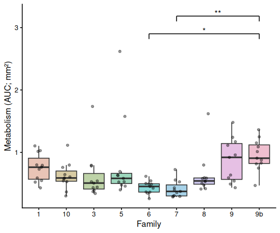
14 Save Output Data
write_csv(auc_all,      file.path(out_dir, "auc_all_metrics.csv"))
write_csv(auc_summary,  file.path(out_dir, "auc_summary.csv"))

if (nrow(metabolism_df) > 0)
  write_csv(metabolism_df,
            file.path(out_dir, "metabolism.csv"))

stats_compiled <- map_dfr(metrics_to_test, function(met) {
  bind_rows(
    stats_results[[met]]$pairs_full %>%
      mutate(comparison = "family:treatment"),
    stats_results[[met]]$pairs_family %>%
      mutate(comparison = "family"),
    stats_results[[met]]$pairs_trt %>%
      mutate(comparison = "treatment")
  ) %>% mutate(metric = met)
})

write_csv(stats_compiled,
          file.path(out_dir, "pairwise_stats.csv"))

message("Output files written to: ", out_dir)