INTRO
M.gigas oysters from nine different USDA families were subjected to heat stress @ 33oC in a large, upright incubator. Oysters were submerged in seawater in 24-well plates. Survivorship was assessed periodically over a 72hr period.
Well temps were spot checked at each time point using an infrared thermometer. Temps were generally in a range from 32-38oC over the course of the entire experiment. Wells closer to the door were generally cooler than those further back in the incubator, which may have contributed to some of the variability in survivorship observed across families.
Plates were arranged in a single layer (i.e. not stacked) in the incubator and were rotated after each time point to minimize any potential effects of well position on survivorship.
The post below was knitted from 00.00-mgig-heat-survivorship-20260511.Rmd (GitHub).
1 BACKGROUND
1.1 SETUP
1.1.1 Load packages
library(readr)
library(dplyr)
library(survival)
library(survminer)
library(ggplot2)

knitr::opts_chunk$set(
  echo = TRUE,         # Display code chunks
  eval = TRUE,        # Evaluate code chunks
  warning = FALSE,     # Hide warnings
  message = FALSE,     # Hide messages
  comment = "",         # Prevents appending '##' to beginning of lines in code output
  results = 'hold'     # Holds output so it's all printed together after code chunk
)
1.1.2 Read in and view raw data
survivorship_raw <- read_csv(
    "../heat-survivorship/20260511-33C-USDA-families/survivorship.csv",
    show_col_types = FALSE
)

# Preview newly created object
cat("\n=== survivorship_raw: str() ===\n")
str(survivorship_raw)
=== survivorship_raw: str() ===
spc_tbl_ [1,080 × 10] (S3: spec_tbl_df/tbl_df/tbl/data.frame)
$ plate_ID : chr [1:1080] "plate-A" "plate-A" "plate-A" "plate-A" ...
$ plate_well : chr [1:1080] "A01" "A02" "A03" "A04" ...
$ individual_id : num [1:1080] 1 2 3 4 5 6 7 8 9 10 ...
$ familly_id.group : chr [1:1080] "3" "3" "3" "3" ...
$ timepoint_count : num [1:1080] 0 0 0 0 0 0 0 0 0 0 ...
$ timepoint_hrs : num [1:1080] 0 0 0 0 0 0 0 0 0 0 ...
$ alive.measurement: logi [1:1080] TRUE TRUE TRUE TRUE TRUE TRUE ...
$ date : num [1:1080] 20260511 20260511 20260511 20260511 20260511 ...
$ time : 'hms' num [1:1080] 12:30:00 12:30:00 12:30:00 12:30:00 ...
..- attr(*, "units")= chr "secs"
$ notes : logi [1:1080] NA NA NA NA NA NA ...
- attr(*, "spec")=
.. cols(
.. plate_ID = col_character(),
.. plate_well = col_character(),
.. individual_id = col_double(),
.. familly_id.group = col_character(),
.. timepoint_count = col_double(),
.. timepoint_hrs = col_double(),
.. alive.measurement = col_logical(),
.. date = col_double(),
.. time = col_time(format = ""),
.. notes = col_logical()
.. )
- attr(*, "problems")=<pointer: 0x5a6584bbccc0> 1.2 ANALYSIS
1.2.1 Clean and standardize columns used for survival analysis
survivorship_clean <- survivorship_raw %>%
    mutate(
        individual_id = as.character(individual_id),
        family_group = as.character(`familly_id.group`),
        timepoint_hrs = as.numeric(timepoint_hrs),
        alive_chr = toupper(trimws(as.character(`alive.measurement`))),
        alive = case_when(
            alive_chr %in% c("TRUE", "T", "1", "YES", "Y") ~ TRUE,
            alive_chr %in% c("FALSE", "F", "0", "NO", "N") ~ FALSE,
            TRUE ~ NA
        )
    ) %>%
    select(
        individual_id,
        family_group,
        timepoint_count,
        timepoint_hrs,
        alive,
        date,
        time,
        everything()
    )

# Preview newly created object
cat("\n=== survivorship_clean: str() ===\n")
str(survivorship_clean)
cat("\n=== survivorship_clean: summary(alive) ===\n")
summary(survivorship_clean$alive)
=== survivorship_clean: str() ===
tibble [1,080 × 13] (S3: tbl_df/tbl/data.frame)
$ individual_id : chr [1:1080] "1" "2" "3" "4" ...
$ family_group : chr [1:1080] "3" "3" "3" "3" ...
$ timepoint_count : num [1:1080] 0 0 0 0 0 0 0 0 0 0 ...
$ timepoint_hrs : num [1:1080] 0 0 0 0 0 0 0 0 0 0 ...
$ alive : logi [1:1080] TRUE TRUE TRUE TRUE TRUE TRUE ...
$ date : num [1:1080] 20260511 20260511 20260511 20260511 20260511 ...
$ time : 'hms' num [1:1080] 12:30:00 12:30:00 12:30:00 12:30:00 ...
..- attr(*, "units")= chr "secs"
$ plate_ID : chr [1:1080] "plate-A" "plate-A" "plate-A" "plate-A" ...
$ plate_well : chr [1:1080] "A01" "A02" "A03" "A04" ...
$ familly_id.group : chr [1:1080] "3" "3" "3" "3" ...
$ alive.measurement: logi [1:1080] TRUE TRUE TRUE TRUE TRUE TRUE ...
$ notes : logi [1:1080] NA NA NA NA NA NA ...
$ alive_chr : chr [1:1080] "TRUE" "TRUE" "TRUE" "TRUE" ...
=== survivorship_clean: summary(alive) ===
Mode FALSE TRUE
logical 683 397 1.2.2 Reduce repeated observations to one survival row per individual
individual_survival <- survivorship_clean %>%
    filter(!is.na(individual_id), !is.na(timepoint_hrs), !is.na(alive)) %>%
    arrange(individual_id, timepoint_hrs) %>%
    group_by(individual_id) %>%
    summarise(
        family_group = first(family_group[!is.na(family_group)]),
        event = if_else(any(!alive), 1L, 0L),
        time_to_event = {
            if (any(!alive)) {
                min(timepoint_hrs[!alive])
            } else {
                max(timepoint_hrs)
            }
        },
        n_observations = n(),
        .groups = "drop"
    )

# Preview newly created object
cat("\n=== individual_survival: str() ===\n")
str(individual_survival)
cat("\n=== individual_survival: summary(time_to_event) ===\n")
summary(individual_survival$time_to_event)
cat("\n=== individual_survival: table(event) ===\n")
table(individual_survival$event)
=== individual_survival: str() ===
tibble [108 × 5] (S3: tbl_df/tbl/data.frame)
$ individual_id : chr [1:108] "1" "10" "100" "101" ...
$ family_group : chr [1:108] "3" "3" "6" "6" ...
$ event : int [1:108] 1 1 1 1 1 1 1 1 1 1 ...
$ time_to_event : num [1:108] 48 48 22 43 27 27 22 43 22 43 ...
$ n_observations: int [1:108] 10 10 10 10 10 10 10 10 10 10 ...
=== individual_survival: summary(time_to_event) ===
Min. 1st Qu. Median Mean 3rd Qu. Max.
22.00 24.83 43.00 36.42 43.00 67.00
=== individual_survival: table(event) ===
0 1
1 107 1.2.3 Create Surv object and fit Kaplan-Meier models
surv_object <- with(individual_survival, Surv(time = time_to_event, event = event))

km_fit_overall <- survfit(surv_object ~ 1, data = individual_survival)
km_fit_by_family <- survfit(surv_object ~ family_group, data = individual_survival)

# Preview newly created objects
cat("\n=== km_fit_overall ===\n")
print(km_fit_overall)
cat("\n=== km_fit_by_family ===\n")
print(km_fit_by_family)
cat("\n=== km_fit_overall: str() ===\n")
str(km_fit_overall)
cat("\n=== km_fit_by_family: str() ===\n")
str(km_fit_by_family)
=== km_fit_overall ===
Call: survfit(formula = surv_object ~ 1, data = individual_survival)
n events median 0.95LCL 0.95UCL
[1,] 108 107 43 27 43
=== km_fit_by_family ===
Call: survfit(formula = surv_object ~ family_group, data = individual_survival)
n events median 0.95LCL 0.95UCL
family_group=1 12 12 43.0 27.0 NA
family_group=10 12 12 22.0 22.0 NA
family_group=3 12 12 35.0 27.0 NA
family_group=5 12 12 43.0 43.0 NA
family_group=6 12 12 27.0 22.0 NA
family_group=7 12 12 24.8 22.0 NA
family_group=8 12 11 27.0 24.8 NA
family_group=9 12 12 43.0 43.0 NA
family_group=9b 12 12 43.0 43.0 NA
=== km_fit_overall: str() ===
List of 17
$ n : int 108
$ time : num [1:8] 22 24.8 27 43 45 ...
$ n.risk : num [1:8] 108 89 77 57 17 16 12 8
$ n.event : num [1:8] 19 12 20 40 1 4 4 7
$ n.censor : num [1:8] 0 0 0 0 0 0 0 1
$ surv : num [1:8] 0.824 0.713 0.528 0.157 0.148 ...
$ std.err : num [1:8] 0.0445 0.0611 0.091 0.2226 0.2307 ...
$ cumhaz : num [1:8] 0.176 0.311 0.57 1.272 1.331 ...
$ std.chaz : num [1:8] 0.0404 0.0561 0.0807 0.1372 0.1493 ...
$ type : chr "right"
$ logse : logi TRUE
$ conf.int : num 0.95
$ conf.type: chr "log"
$ lower : num [1:8] 0.7553 0.6326 0.4415 0.1017 0.0943 ...
$ upper : num [1:8] 0.899 0.804 0.631 0.244 0.233 ...
$ t0 : num 0
$ call : language survfit(formula = surv_object ~ 1, data = individual_survival)
- attr(*, "class")= chr "survfit"
=== km_fit_by_family: str() ===
List of 18
$ n : int [1:9] 12 12 12 12 12 12 12 12 12
$ time : num [1:37] 22 27 43 45 48 ...
$ n.risk : num [1:37] 12 11 8 3 2 1 12 5 2 1 ...
$ n.event : num [1:37] 1 3 5 1 1 1 7 3 1 1 ...
$ n.censor : num [1:37] 0 0 0 0 0 0 0 0 0 0 ...
$ surv : num [1:37] 0.9167 0.6667 0.25 0.1667 0.0833 ...
$ std.err : num [1:37] 0.087 0.204 0.5 0.645 0.957 ...
$ cumhaz : num [1:37] 0.0833 0.3561 0.9811 1.3144 1.8144 ...
$ std.chaz : num [1:37] 0.0833 0.1782 0.3315 0.4701 0.6863 ...
$ strata : Named int [1:9] 6 4 5 4 4 4 4 3 3
..- attr(*, "names")= chr [1:9] "family_group=1" "family_group=10" "family_group=3" "family_group=5" ...
$ type : chr "right"
$ logse : logi TRUE
$ conf.int : num 0.95
$ conf.type: chr "log"
$ lower : num [1:37] 0.7729 0.4468 0.0938 0.047 0.0128 ...
$ upper : num [1:37] 1 0.995 0.666 0.591 0.544 ...
$ t0 : num 0
$ call : language survfit(formula = surv_object ~ family_group, data = individual_survival)
- attr(*, "class")= chr "survfit"1.2.4 Perform log-rank test to compare survival between families
logrank_test <- survdiff(surv_object ~ family_group, data = individual_survival)

# Display test results
cat("\n=== Log-rank test: survdiff() output ===\n")
print(logrank_test)

# Extract and report key statistics
cat("\n=== Log-Rank Test Summary ===\n")
cat("Chi-square statistic:", logrank_test$chisq, "\n")
cat("Degrees of freedom:", length(logrank_test$n) - 1, "\n")
cat("p-value:", 1 - pchisq(logrank_test$chisq, df = length(logrank_test$n) - 1), "\n")
cat("\nInterpretation:\n")
p_val <- 1 - pchisq(logrank_test$chisq, df = length(logrank_test$n) - 1)
if (p_val < 0.05) {
  cat("p < 0.05: Family groups show SIGNIFICANTLY DIFFERENT survival (reject null hypothesis)\n")
} else {
  cat("p >= 0.05: No significant difference in survival detected between family groups\n")
}
=== Log-rank test: survdiff() output ===
Call:
survdiff(formula = surv_object ~ family_group, data = individual_survival)
N Observed Expected (O-E)^2/E (O-E)^2/V
family_group=1 12 12 14.28 0.365 0.744
family_group=10 12 12 5.52 7.593 12.784
family_group=3 12 12 13.34 0.134 0.259
family_group=5 12 12 19.47 2.869 6.823
family_group=6 12 12 7.81 2.241 3.934
family_group=7 12 12 6.46 4.754 8.000
family_group=8 12 11 7.50 1.637 2.650
family_group=9 12 12 17.43 1.690 3.802
family_group=9b 12 12 15.18 0.667 1.426
Chisq= 38.3 on 8 degrees of freedom, p= 7e-06
=== Log-Rank Test Summary ===
Chi-square statistic: 38.31314
Degrees of freedom: 8
p-value: 6.588796e-06
Interpretation:
p < 0.05: Family groups show SIGNIFICANTLY DIFFERENT survival (reject null hypothesis)1.2.5 Pairwise log-rank tests with BH correction
pairwise_results <- pairwise_survdiff(
    Surv(time_to_event, event) ~ family_group,
    data = individual_survival,
    p.adjust.method = "BH"
)

cat("\n=== Pairwise log-rank test (BH-adjusted p-values) ===\n")
print(pairwise_results)

# Extract and display only significant pairs
p_mat <- pairwise_results$p.value
sig_pairs <- which(p_mat <= 0.05, arr.ind = TRUE)

cat("\n=== Significant pairwise comparisons (BH-adjusted p <= 0.05) ===\n")
if (nrow(sig_pairs) == 0) {
    cat("No significant pairwise differences found.\n")
} else {
    sig_df <- data.frame(
        group1      = rownames(p_mat)[sig_pairs[, 1]],
        group2      = colnames(p_mat)[sig_pairs[, 2]],
        p_adjusted  = p_mat[sig_pairs]
    )
    print(sig_df)
}
=== Pairwise log-rank test (BH-adjusted p-values) ===
Pairwise comparisons using Log-Rank test
data: individual_survival and family_group
1 10 3 5 6 7 8 9
10 0.0333 - - - - - - -
3 0.8810 0.0333 - - - - - -
5 0.2411 0.0051 0.2382 - - - - -
6 0.0549 0.2681 0.1482 0.0051 - - - -
7 0.0251 0.5335 0.0532 0.0038 0.6378 - - -
8 0.1918 0.0846 0.3170 0.0333 0.8543 0.7041 - -
9 0.4492 0.0038 0.2858 0.5155 0.0038 0.0038 0.0142 -
9b 0.9547 0.0075 0.8835 0.1918 0.0075 0.0038 0.0142 0.3198
P value adjustment method: BH
=== Significant pairwise comparisons (BH-adjusted p <= 0.05) ===
group1 group2 p_adjusted
1 10 1 0.033324135
2 7 1 0.025143399
3 3 10 0.033324135
4 5 10 0.005050921
5 9 10 0.003843674
6 9b 10 0.007545462
7 6 5 0.005050921
8 7 5 0.003843674
9 8 5 0.033324135
10 9 6 0.003843674
11 9b 6 0.007545462
12 9 7 0.003843674
13 9b 7 0.003843674
14 9 8 0.014195943
15 9b 8 0.0141959431.2.6 Convert Kaplan-Meier fit to plotting data frames
km_overall_df <- bind_rows(
    data.frame(
        time = 0,
        surv = 1,
        n_risk = km_fit_overall$n,
        n_event = 0,
        n_censor = 0
    ),
    summary(km_fit_overall) %>%
        with(
            data.frame(
                time = time,
                surv = surv,
                n_risk = n.risk,
                n_event = n.event,
                n_censor = n.censor
            )
        )
) %>%
    arrange(time)

km_family_df <- bind_rows(
    data.frame(
        time = 0,
        surv = 1,
        n_risk = as.numeric(km_fit_by_family$n),
        n_event = 0,
        n_censor = 0,
        strata = names(km_fit_by_family$strata)
    ),
    summary(km_fit_by_family) %>%
        with(
            data.frame(
                time = time,
                surv = surv,
                n_risk = n.risk,
                n_event = n.event,
                n_censor = n.censor,
                strata = strata
            )
        )
) %>%
    mutate(family_group = sub("^family_group=", "", strata)) %>%
    arrange(family_group, time)

# Preview newly created objects
cat("\n=== km_overall_df: head() ===\n")
print(head(km_overall_df))
cat("\n=== km_overall_df: str() ===\n")
str(km_overall_df)

cat("\n=== km_family_df: head() ===\n")
print(head(km_family_df))
cat("\n=== km_family_df: str() ===\n")
str(km_family_df)
=== km_overall_df: head() ===
time surv n_risk n_event n_censor
1 0.00 1.0000000 108 0 0
2 22.00 0.8240741 108 19 0
3 24.83 0.7129630 89 12 0
4 27.00 0.5277778 77 20 0
5 43.00 0.1574074 57 40 0
6 45.00 0.1481481 17 1 0
=== km_overall_df: str() ===
'data.frame': 9 obs. of 5 variables:
$ time : num 0 22 24.8 27 43 ...
$ surv : num 1 0.824 0.713 0.528 0.157 ...
$ n_risk : num 108 108 89 77 57 17 16 12 8
$ n_event : num 0 19 12 20 40 1 4 4 7
$ n_censor: num 0 0 0 0 0 0 0 0 1
=== km_family_df: head() ===
time surv n_risk n_event n_censor strata family_group
1 0 1.00000000 12 0 0 family_group=1 1
2 22 0.91666667 12 1 0 family_group=1 1
3 27 0.66666667 11 3 0 family_group=1 1
4 43 0.25000000 8 5 0 family_group=1 1
5 45 0.16666667 3 1 0 family_group=1 1
6 48 0.08333333 2 1 0 family_group=1 1
=== km_family_df: str() ===
'data.frame': 45 obs. of 7 variables:
$ time : num 0 22 27 43 45 ...
$ surv : num 1 0.917 0.667 0.25 0.167 ...
$ n_risk : num 12 12 11 8 3 2 1 12 12 5 ...
$ n_event : num 0 1 3 5 1 1 1 0 7 3 ...
$ n_censor : num 0 0 0 0 0 0 0 0 0 0 ...
$ strata : chr "family_group=1" "family_group=1" "family_group=1" "family_group=1" ...
$ family_group: chr "1" "1" "1" "1" ...1.3 PLOTS
1.3.1 Plot Kaplan-Meier curves
1.3.1.1 Families
ggplot(km_family_df, aes(x = time, y = surv, color = family_group)) +
    geom_step(linewidth = 1.0) +
    labs(
        title = "Kaplan-Meier Survival Curves by Family Group",
        x = "Time (hours)",
        y = "Survival probability",
        color = "Family group"
    ) +
    ylim(0, 1) +
    theme_minimal(base_size = 12)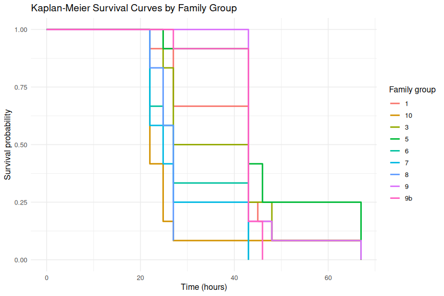
DISCUSSION
There were significant differences in survivorship between the different families of M.gigas oysters under heat stress at 33oC. The log-rank test indicated that family groups had significantly different survival curves (p < 0.05). Pairwise comparisons with BH correction revealed specific family pairs that differed significantly in survival.
| group1 | group2 | p_adjusted |
|---|---|---|
| 10 | 1 | 0.033324135 |
| 7 | 1 | 0.025143399 |
| 3 | 10 | 0.033324135 |
| 5 | 10 | 0.005050921 |
| 9 | 10 | 0.003843674 |
| 9b | 10 | 0.007545462 |
| 6 | 5 | 0.005050921 |
| 7 | 5 | 0.003843674 |
| 8 | 5 | 0.033324135 |
| 9 | 6 | 0.003843674 |
| 9b | 6 | 0.007545462 |
| 9 | 7 | 0.003843674 |
| 9b | 7 | 0.003843674 |
| 9 | 8 | 0.014195943 |
| 9b | 8 | 0.014195943 |