Resazurin Assays - USDA M.gigas Families in Response to Temperature Stress

INTRO

Twenty adult oysters from each of four different USDA families (1, 5, 7, & 9) were subjected to acute heat stress at 36^oC for four hours in an upright incubator. Oysters were photographed for measurement and then submerged in ~70mL of freshly prepared resazuring solution in plastic drink cups. Resazurin fluorescence was measured by extracting 200uL from each cup and placing in a 96-well plate, then measuring fluorescence in a Synergy HTX plate reader (Agilent).

Image of undergrad loading tray of cups containing oysters and resazurin into incubator in Graham Young’s lab

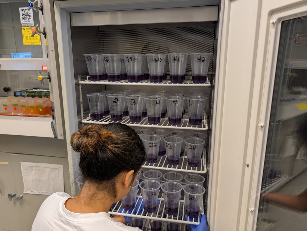
To speed up sampling and reduce the amount of time cups were out of the incubator, sampling was periodcially divided between two people and two plates (i.e. half the samples collected into plate B, the other half into plate C).

[!NOTE] Based on our experience with resazurin fluorescence stability and the sheer number of samples being handled, resazurin fluorescence was not measured immediately. Plates were measured when time was available, however, no plates sat for longer than 30 minutes at room temperature.

Resazurin temperatures were measured with an infrared thermometer over the course of the experiment:

Timepoint (hrs)	Temp_range (C)
0	18
0.5	23-29
1	27-29
1.5	29-31
2	30-32
2.5	31.5-32.5
3	31.5-32.5
3.5	31-32.5
4	31.5-33

Notebook was knitted from 01.00-resazurin-20260713-mgig-36C.Rmd (GitHub).

RESULTS

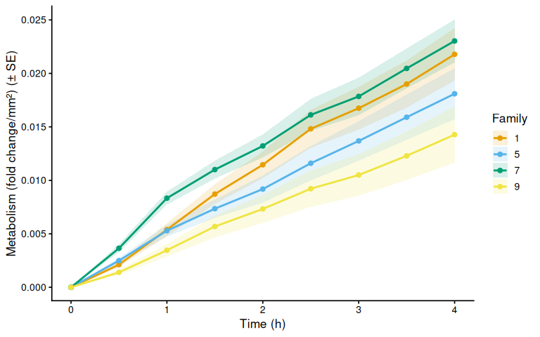
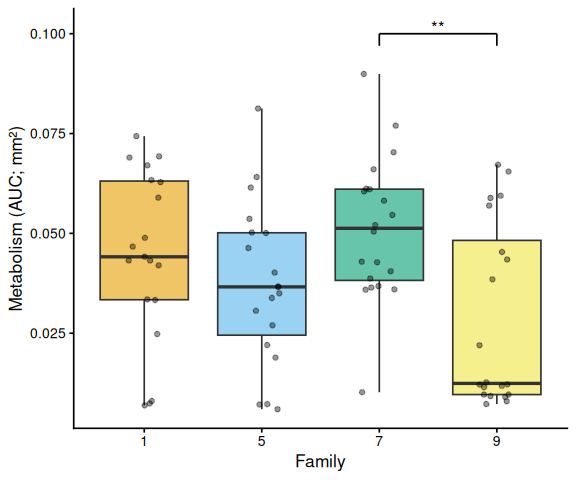
Family significantly affected size-normalized metabolic rate (AUC ANOVA: F=4.37, p=0.0069), with a significant time × family interaction in the time-series model (LME: p=0.0006). Family 7 had the highest mean metabolic activity and Family 9 the lowest; this contrast was the only significant pairwise difference (Tukey: p=0.0051). The divergence emerged by 1.5 h and strengthened through 4 h (p=0.0002). Families 1 and 5 were intermediate and not significantly different from any other family.

Mean area-under-the-curve (AUC) of blank-corrected metabolism (fold change / mm² shell area) per family across the 4 h heat stress period.

Family	n	Mean AUC	SE
7	20	0.0511	0.0040
1	19	0.0446	0.0049
5	19	0.0373	0.0047
9	20	0.0285	0.0051

Two wells were excluded due to a cup mix-up (samples 70 and 71: one cup contained two oysters, the other none).

---

1 Background

To speed up sampling and reduce the amount of time cups were out of the incubator, sampling was periodcially divided between two people and two plates (i.e. half the samples collected into plate B, the other half into plate C).

\[!NOTE\] Based on our experience with resazurin fluorescence stability and the sheer number of samples being handled, resazurin fluorescence was not measured immediately. Plates were measured when time was available, however, no plates sat for longer than 30 minutes at room temperature.

Resazurin temperatures were measured with an infrared thermometer over the course of the experiment:

Timepoint (hrs)	Temp_range (C)
0	18
0.5	23-29
1	27-29
1.5	29-31
2	30-32
2.5	31.5-32.5
3	31.5-32.5
3.5	31-32.5
4	31.5-33

See Resazurin/data/20260713-mgig-36C/README.md for full experimental notes.

1.1 Expected inputs

Path	Description
Resazurin/data/20260713-mgig-36C/plate-*-T*.txt	Plate reader fluorescence exports (one file per plate per timepoint)
Resazurin/data/20260713-mgig-36C/layout.csv	Well metadata: plate ID, well ID, blank flag, family groups, sample IDs, area measurements (mm², from ImageJ)

1.2 Expected outputs

All outputs are written to Resazurin/outputs/01.00-resazurin-20260713-mgig-36C/.

File	Description
figures/	All plots generated by this script
auc_all_metrics.csv	Per-individual AUC values for every active measurement metric
auc_summary.csv	Group-level AUC summary statistics (mean, SD, SE, median)
metabolism.csv	Full per-well per-timepoint metabolism data frame
pairwise_stats.csv	Tukey-adjusted pairwise comparisons from AUC linear models

2 Setup

2.1 Knitr options

knitr::opts_chunk$set(
  echo = TRUE,         # Display code chunks
  eval = TRUE,        # Evaluate code chunks
  warning = FALSE,     # Hide warnings
  message = FALSE,     # Hide messages
  comment = "",         # Prevents appending '##' to beginning of lines in code output
  results = 'hold'     # Holds output so it's all printed together after code chunk
)

2.2 Load libraries

library(tidyverse)
library(pracma)       # trapz()
library(lme4)
library(lmerTest)
library(emmeans)
library(multcompView)
library(cowplot)
library(colorspace)   # qualitative_hcl() for large palettes

3 Helper Functions

normalize_well_id <- function(x) {
  x <- toupper(trimws(x))
  valid <- str_detect(x, "^[A-Z]+[0-9]+$")
  out <- rep(NA_character_, length(x))
  if (!any(valid)) return(out)
  m <- str_match(x[valid], "^([A-Z]+)([0-9]+)$")
  out[valid] <- paste0(m[, 2], as.integer(m[, 3]))
  out
}

parse_time_hr <- function(path) {
  hit <- str_match(basename(path),
                   "(?i)-T([0-9]+(?:\\.[0-9]+)?)\\.txt$")
  as.numeric(hit[, 2])
}

parse_plate_id <- function(path) {
  hit <- str_match(basename(path),
    "(?i)^plate-([A-Za-z0-9-]+)-T[0-9]+(?:\\.[0-9]+)?\\.txt$")
  id <- hit[, 2]
  ifelse(is.na(id), "unknown", id)
}

extract_results_block <- function(lines) {
  results_idx <- which(trimws(lines) == "Results")
  if (length(results_idx) == 0) stop("No Results section found")
  idx <- results_idx[1]
  header_tokens <- str_split(lines[idx + 1], "\\t")[[1]] |> trimws()
  col_ids <- header_tokens[
    header_tokens != "" & str_detect(header_tokens, "^[0-9]+$")]
  j <- idx + 2
  data_lines <- character()
  while (j <= length(lines)) {
    line <- lines[j]
    if (trimws(line) == "") break
    if (!str_detect(line, "^[A-Za-z]\\t")) break
    data_lines <- c(data_lines, line)
    j <- j + 1
  }
  list(col_ids = col_ids, data_lines = data_lines)
}

parse_plate_export <- function(path) {
  lines <- readLines(path, warn = FALSE)
  res <- extract_results_block(lines)

  map_dfr(res$data_lines, function(line) {
    tokens <- str_split(line, "\\t")[[1]] |> trimws()
    tokens <- tokens[tokens != ""]
    row_letter <- tokens[1]
    nums <- suppressWarnings(as.numeric(tokens[-1]))
    valid_idx <- which(!is.na(nums))
    if (length(valid_idx) == 0) return(tibble())
    vals <- nums[valid_idx]
    n <- min(length(vals), length(res$col_ids))
    tibble(
      row_id  = toupper(row_letter),
      col_id  = as.integer(res$col_ids[seq_len(n)]),
      well_id = normalize_well_id(
        paste0(toupper(row_letter), res$col_ids[seq_len(n)])),
      value   = vals[seq_len(n)]
    )
  }) %>%
    mutate(
      plate_id = str_to_lower(parse_plate_id(path)),
      time_hr  = parse_time_hr(path)
    )
}

trapezoid_auc <- function(time_hr, value) {
  ok <- is.finite(time_hr) & is.finite(value)
  t <- time_hr[ok]
  v <- value[ok]
  if (length(t) < 2) return(NA_real_)
  ord <- order(t)
  t <- t[ord]; v <- v[ord]
  sum(diff(t) * (head(v, -1) + tail(v, -1)) / 2)
}

# Shared helper: extract display unit string from a measurement column name.
# e.g. "area_mm2_measurement" -> "mm²", "weight_mg_measurement" -> "mg"
parse_meas_unit <- function(col_name) {
  unit_raw <- col_name |>
    str_remove("^metabolism_per_") |>
    str_remove("_measurement$") |>
    str_extract("[^_]+$")
  case_when(
    unit_raw == "mm2" ~ "mm²",
    unit_raw == "cm2" ~ "cm²",
    unit_raw == "mm3" ~ "mm³",
    unit_raw == "cm3" ~ "cm³",
    TRUE              ~ unit_raw
  )
}

# y-axis label for metabolism line plots: "fold change/mm²"
metabolism_y_label <- function(col_name) {
  paste0("Metabolism (fold change/", parse_meas_unit(col_name), ")")
}

# y-axis label for AUC box plots: "Metabolism (AUC; mm²)"
auc_y_label <- function(metric_name) {
  paste0("Metabolism (AUC; ", parse_meas_unit(metric_name), ")")
}

4 Load Data

4.1 Plate export files

proj_root <- rprojroot::find_rstudio_root_file()
data_dir  <- file.path(proj_root, "Resazurin", "data", "20260713-mgig-36C")
out_dir   <- file.path(proj_root, "Resazurin", "outputs",
                        "01.00-resazurin-20260713-mgig-36C")
fig_dir   <- file.path(out_dir, "figures")

dir.create(fig_dir, recursive = TRUE, showWarnings = FALSE)
dir.create(out_dir, recursive = TRUE, showWarnings = FALSE)

plate_files <- list.files(
  data_dir,
  pattern = "(?i)^plate-.*-T[0-9]+(?:\\.[0-9]+)?\\.txt$",
  full.names = TRUE
)

plate_raw <- map_dfr(plate_files, function(path) {
  tryCatch(parse_plate_export(path),
           error = function(e) {
             message("Parse error in ", basename(path), ": ", e$message)
             tibble()
           })
})

str(plate_raw)

tibble [1,248 × 6] (S3: tbl_df/tbl/data.frame)
 $ row_id  : chr [1:1248] "A" "A" "A" "A" ...
 $ col_id  : int [1:1248] 1 2 3 4 5 6 7 8 9 10 ...
 $ well_id : chr [1:1248] "A1" "A2" "A3" "A4" ...
 $ value   : num [1:1248] 596 597 605 613 601 626 626 626 610 636 ...
 $ plate_id: chr [1:1248] "a" "a" "a" "a" ...
 $ time_hr : num [1:1248] 0 0 0 0 0 0 0 0 0 0 ...

4.2 Plate consistency check

Checks that every plate has the same number of wells at every timepoint. The expected well count is the mode across all plate × timepoint reads. Any plate with at least one deviating read is flagged and dropped entirely before any further analysis — removing only the aberrant timepoint would break the fold-change baseline calculation.

well_counts <- plate_raw %>%
  group_by(plate_id, time_hr) %>%
  summarise(n_wells = n_distinct(well_id), .groups = "drop")

expected_n_wells <- as.integer(
  names(which.max(table(well_counts$n_wells)))
)

inconsistent_reads <- well_counts %>%
  filter(n_wells != expected_n_wells) %>%
  arrange(plate_id, time_hr)

inconsistent_plate_ids <- unique(inconsistent_reads$plate_id)

if (nrow(inconsistent_reads) > 0) {
  cat("**Plate consistency check FAILED.**",
      "Expected", expected_n_wells, "wells per plate-timepoint read.",
      length(inconsistent_plate_ids),
      "plate(s) have at least one deviating read and are excluded",
      "from all analyses:\n\n")
  cat(knitr::kable(
    inconsistent_reads,
    col.names = c("Plate", "Time (h)", "Wells read"),
    caption   = paste("Expected:", expected_n_wells, "wells per read")
  ), sep = "\n")
  cat("\n")
  plate_raw <- plate_raw %>%
    filter(!plate_id %in% inconsistent_plate_ids)
  message(length(inconsistent_plate_ids),
          " plate(s) removed from plate_raw: ",
          paste(inconsistent_plate_ids, collapse = ", "))
} else {
  cat("Plate consistency check passed: all",
      n_distinct(well_counts$plate_id), "plates have",
      expected_n_wells, "wells at every timepoint.\n")
}

Plate consistency check passed: all 3 plates have 96 wells at every timepoint.

4.3 Layout file

layout_path <- file.path(data_dir, "layout.csv")

layout_raw <- read_csv(layout_path,
                       col_types = cols(.default = "c"),
                       show_col_types = FALSE)

# Standardise column names to snake_case
names(layout_raw) <- names(layout_raw) |>
  str_to_lower() |>
  str_replace_all("[^a-z0-9]+", "_") |>
  str_replace_all("_+", "_") |>
  str_replace("_$", "")

# Normalise plate_id to match plate file ids (strip "plate-" prefix)
layout_clean <- layout_raw %>%
  mutate(
    plate_id = str_remove(str_to_lower(plate_id), "^plate-"),
    well_id  = normalize_well_id(plate_well),
    is_blank = if ("is_blank" %in% names(layout_raw))
      toupper(trimws(is_blank)) %in% c("TRUE", "T", "1", "YES", "Y")
    else
      FALSE
  )

found_exclude_col <- intersect(
  c("exclude_from_analysis", "exclude", "omit", "not_analyzed"),
  names(layout_clean)
)[1]
layout_clean <- layout_clean %>%
  mutate(
    exclude_from_analysis = if (!is.na(found_exclude_col))
      toupper(trimws(.data[[found_exclude_col]])) %in%
        c("TRUE", "T", "1", "YES", "Y")
    else
      FALSE
  )

# Identify measurement columns and group columns
measurement_cols <- names(layout_clean)[
  str_detect(names(layout_clean), "_measurement$")]
group_cols <- names(layout_clean)[
  str_detect(names(layout_clean), "_group$")]

# Cast measurement columns to numeric
layout_clean <- layout_clean %>%
  mutate(across(all_of(measurement_cols),
                ~ suppressWarnings(as.numeric(.x))))

# Determine which measurement columns actually contain finite data
active_meas_cols <- measurement_cols[
  sapply(measurement_cols, function(col)
    any(is.finite(layout_clean[[col]]), na.rm = TRUE))]

# Normalise group values to lowercase so they match colour scale definitions
layout_clean <- layout_clean %>%
  mutate(across(all_of(group_cols),
                ~ str_to_lower(trimws(as.character(.x)))))

message("Group columns: ", paste(group_cols, collapse = ", "))
message("Active measurement columns: ",
        paste(active_meas_cols, collapse = ", "))

str(layout_clean)

tibble [235 × 14] (S3: tbl_df/tbl/data.frame)
 $ plate_id             : chr [1:235] "a" "a" "a" "a" ...
 $ plate_well           : chr [1:235] "A01" "A02" "A03" "A04" ...
 $ is_blank             : logi [1:235] FALSE FALSE FALSE FALSE FALSE FALSE ...
 $ family_id_group      : chr [1:235] "7" "5" "1" "9" ...
 $ sample_id_group      : chr [1:235] "1" "2" "3" "4" ...
 $ treatment_group      : chr [1:235] NA NA NA NA ...
 $ exclude_from_analysis: logi [1:235] FALSE FALSE FALSE FALSE FALSE FALSE ...
 $ exclude_reason       : chr [1:235] NA NA NA NA ...
 $ width_mm_measurement : num [1:235] NA NA NA NA NA NA NA NA NA NA ...
 $ length_mm_measurement: num [1:235] NA NA NA NA NA NA NA NA NA NA ...
 $ weight_mg_measurement: num [1:235] NA NA NA NA NA NA NA NA NA NA ...
 $ area_mm2_measurement : num [1:235] 538 586 713 757 823 ...
 $ imagej_id            : chr [1:235] "2" "4" "1" "1" ...
 $ well_id              : chr [1:235] "A1" "A2" "A3" "A4" ...

5 Merge Plate Data with Layout

dat <- plate_raw %>%
  left_join(
    layout_clean %>%
      select(plate_id, well_id, is_blank, exclude_from_analysis,
             any_of("exclude_reason"),
             all_of(group_cols), all_of(measurement_cols)),
    by = c("plate_id", "well_id")
  ) %>%
  mutate(
    is_blank = replace_na(is_blank, FALSE),
    exclude_from_analysis = replace_na(exclude_from_analysis, FALSE)
  )

str(dat)

tibble [1,248 × 16] (S3: tbl_df/tbl/data.frame)
 $ row_id               : chr [1:1248] "A" "A" "A" "A" ...
 $ col_id               : int [1:1248] 1 2 3 4 5 6 7 8 9 10 ...
 $ well_id              : chr [1:1248] "A1" "A2" "A3" "A4" ...
 $ value                : num [1:1248] 596 597 605 613 601 626 626 626 610 636 ...
 $ plate_id             : chr [1:1248] "a" "a" "a" "a" ...
 $ time_hr              : num [1:1248] 0 0 0 0 0 0 0 0 0 0 ...
 $ is_blank             : logi [1:1248] FALSE FALSE FALSE FALSE FALSE FALSE ...
 $ exclude_from_analysis: logi [1:1248] FALSE FALSE FALSE FALSE FALSE FALSE ...
 $ exclude_reason       : chr [1:1248] NA NA NA NA ...
 $ family_id_group      : chr [1:1248] "7" "5" "1" "9" ...
 $ sample_id_group      : chr [1:1248] "1" "2" "3" "4" ...
 $ treatment_group      : chr [1:1248] NA NA NA NA ...
 $ width_mm_measurement : num [1:1248] NA NA NA NA NA NA NA NA NA NA ...
 $ length_mm_measurement: num [1:1248] NA NA NA NA NA NA NA NA NA NA ...
 $ weight_mg_measurement: num [1:1248] NA NA NA NA NA NA NA NA NA NA ...
 $ area_mm2_measurement : num [1:1248] 538 586 713 757 823 ...

6 Raw Fluorescence

6.1 Data frame

# Wells in the plate reader output that have no layout entry get all-NA group
# columns after the join. Keep only wells assigned to at least one group.
active_gc <- intersect(group_cols, names(dat))

raw_df <- dat %>%
  filter(
    !is_blank,
    if (length(active_gc) > 0)
      if_any(all_of(active_gc), ~ !is.na(.))
    else
      TRUE
  ) %>%
  mutate(
    trace_id = if_else(
      !is.na(sample_id_group) & trimws(as.character(sample_id_group)) != "",
      as.character(sample_id_group),
      paste(plate_id, well_id, sep = "_")
    )
  )

families   <- str_sort(unique(na.omit(raw_df$family_id_group)), numeric = TRUE)
treatments <- sort(unique(na.omit(raw_df$treatment_group)))

n_fam <- length(families)
n_trt <- length(treatments)

# Palette strategy:
#   <= 7 groups : Okabe-Ito (gold standard for colorblind-safe figures).
#   >  7 groups : colorspace::qualitative_hcl("Dynamic") scales to any N
#                 using perceptually uniform HCL space — no colour collisions.
# Black (#000000) is excluded from both and reserved for blank wells.
okabe_ito_7 <- c(
  "#E69F00", "#56B4E9", "#009E73", "#F0E442",
  "#0072B2", "#D55E00", "#CC79A7"
)
make_palette <- function(n) {
  if (n == 0L) return(character(0))
  if (n <= length(okabe_ito_7)) return(okabe_ito_7[seq_len(n)])
  colorspace::qualitative_hcl(n, palette = "Dynamic")
}

all_colours   <- make_palette(n_fam + n_trt)
fam_colours   <- setNames(all_colours[seq_len(n_fam)], families)
trt_colours   <- setNames(all_colours[n_fam + seq_len(n_trt)], treatments)

lty_pool <- c("solid", "dashed", "dotted", "dotdash", "longdash")
trt_linetypes <- setNames(
  lty_pool[(seq_len(n_trt) - 1L) %% length(lty_pool) + 1L],
  treatments
)
plate_well_colours <- c(blank = "black", fam_colours)

has_trt <- n_trt > 0

str(raw_df)

tibble [720 × 17] (S3: tbl_df/tbl/data.frame)
 $ row_id               : chr [1:720] "A" "A" "A" "A" ...
 $ col_id               : int [1:720] 1 2 3 4 5 6 7 8 9 10 ...
 $ well_id              : chr [1:720] "A1" "A2" "A3" "A4" ...
 $ value                : num [1:720] 596 597 605 613 601 626 626 626 610 636 ...
 $ plate_id             : chr [1:720] "a" "a" "a" "a" ...
 $ time_hr              : num [1:720] 0 0 0 0 0 0 0 0 0 0 ...
 $ is_blank             : logi [1:720] FALSE FALSE FALSE FALSE FALSE FALSE ...
 $ exclude_from_analysis: logi [1:720] FALSE FALSE FALSE FALSE FALSE FALSE ...
 $ exclude_reason       : chr [1:720] NA NA NA NA ...
 $ family_id_group      : chr [1:720] "7" "5" "1" "9" ...
 $ sample_id_group      : chr [1:720] "1" "2" "3" "4" ...
 $ treatment_group      : chr [1:720] NA NA NA NA ...
 $ width_mm_measurement : num [1:720] NA NA NA NA NA NA NA NA NA NA ...
 $ length_mm_measurement: num [1:720] NA NA NA NA NA NA NA NA NA NA ...
 $ weight_mg_measurement: num [1:720] NA NA NA NA NA NA NA NA NA NA ...
 $ area_mm2_measurement : num [1:720] 538 586 713 757 823 ...
 $ trace_id             : chr [1:720] "1" "2" "3" "4" ...

6.2 Raw fluorescence by plate (including blanks)

p_raw_plates <- dat %>%
  filter(is.finite(time_hr), is.finite(value)) %>%
  mutate(
    colour_group = if_else(is_blank, "blank",
                           coalesce(family_id_group, "sample")),
    trace_id     = paste(plate_id, well_id, sep = "_")
  ) %>%
  ggplot(aes(x = time_hr, y = value,
             group = trace_id, colour = colour_group)) +
  geom_line(alpha = 0.6) +
  geom_point(size = 1, alpha = 0.7) +
  facet_wrap(~ plate_id) +
  scale_colour_manual(
    values   = plate_well_colours,
    name     = "Group",
    breaks   = names(plate_well_colours),
    na.value = "grey80"
  ) +
  labs(x = "Time (h)", y = "Raw fluorescence (RFU)") +
  theme_classic(base_size = 12) +
  theme(strip.background = element_blank(),
        strip.text       = element_text(face = "bold"))

p_raw_plates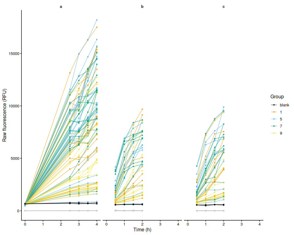

ggsave(file.path(fig_dir, "raw_fluor_by_plate.png"),
       p_raw_plates, width = 10, height = 8)

6.3 Mean raw fluorescence by family

raw_family_summary <- raw_df %>%
  filter(!is.na(family_id_group), !exclude_from_analysis) %>%
  group_by(family_id_group, treatment_group, time_hr) %>%
  summarise(
    mean_fluor = mean(value, na.rm = TRUE),
    se_fluor   = sd(value, na.rm = TRUE) /
      sqrt(sum(!is.na(value))),
    n          = sum(!is.na(value)),
    .groups    = "drop"
  ) %>%
  mutate(group_var = if (has_trt)
    paste(family_id_group, treatment_group, sep = ".")
  else
    family_id_group)

p_raw_mean <- ggplot(raw_family_summary,
    aes(x = time_hr, y = mean_fluor,
        colour = family_id_group,
        group = group_var)) +
  geom_ribbon(aes(ymin = mean_fluor - se_fluor,
                  ymax = mean_fluor + se_fluor,
                  fill = family_id_group),
              alpha = 0.15, colour = NA) +
  geom_line(
    mapping   = if (has_trt) aes(linetype = treatment_group) else NULL,
    linewidth = 1) +
  geom_point(size = 2) +
  scale_colour_manual(values = fam_colours, name = "Family",
                      breaks = families) +
  scale_fill_manual(values = fam_colours, name = "Family",
                    breaks = families) +
  labs(x = "Time (h)", y = "Mean raw fluorescence (RFU ± SE)") +
  theme_classic(base_size = 13) +
  if (has_trt) scale_linetype_manual(values = trt_linetypes, name = "Treatment") else NULL

p_raw_mean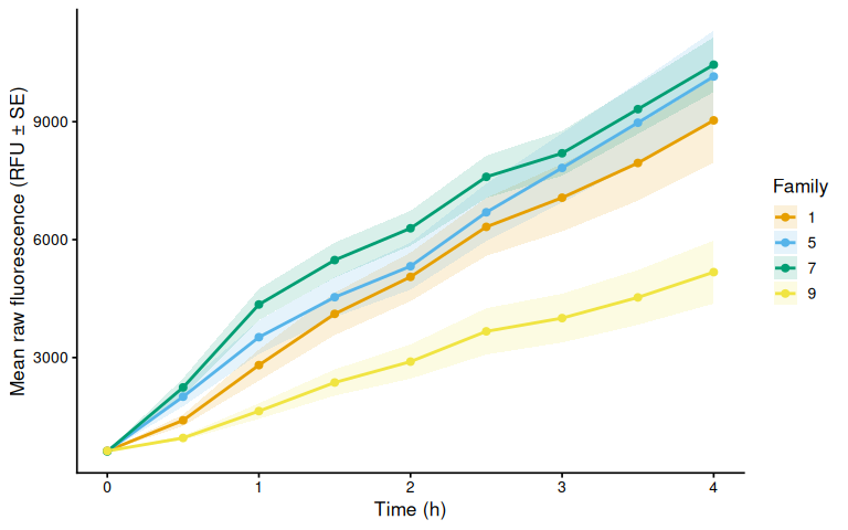

ggsave(file.path(fig_dir, "raw_mean_by_family.png"),
       p_raw_mean, width = 8, height = 5)

6.4 Individual raw fluorescence traces by family

p_raw_by_family <- raw_df %>%
  filter(!is.na(family_id_group)) %>%
  ggplot(aes(x = time_hr, y = value, group = trace_id,
             colour = .data[[if (has_trt) "treatment_group" else "family_id_group"]])) +
  geom_line(alpha = 0.6) +
  geom_point(size = 1.2, alpha = 0.7) +
  facet_wrap(~ family_id_group) +
  scale_colour_manual(
    values = if (has_trt) trt_colours else fam_colours,
    name   = if (has_trt) "Treatment" else "Family",
    breaks = if (has_trt) treatments else families) +
  labs(x = "Time (h)", y = "Raw fluorescence (RFU)") +
  theme_classic(base_size = 12) +
  theme(strip.background = element_blank(),
        strip.text       = element_text(face = "bold"))

p_raw_by_family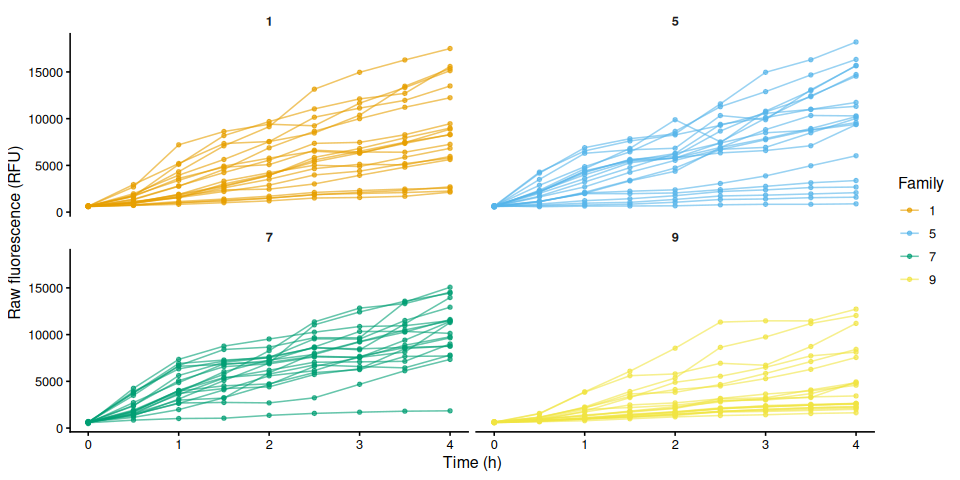

ggsave(file.path(fig_dir, "raw_individual_by_family.png"),
       p_raw_by_family, width = 10, height = 5)

6.5 Individual raw fluorescence traces by treatment

if (has_trt) {
  p_raw_by_treatment <- raw_df %>%
    ggplot(aes(x = time_hr, y = value,
               group = trace_id, colour = family_id_group)) +
    geom_line(alpha = 0.6) +
    geom_point(size = 1.2, alpha = 0.7) +
    facet_wrap(~ treatment_group) +
    scale_colour_manual(values = fam_colours, name = "Family",
                        breaks = families) +
    labs(x = "Time (h)", y = "Raw fluorescence (RFU)") +
    theme_classic(base_size = 12) +
    theme(strip.background = element_blank(),
          strip.text       = element_text(face = "bold"))

  p_raw_by_treatment
  ggsave(file.path(fig_dir, "raw_individual_by_treatment.png"),
         p_raw_by_treatment, width = 10, height = 5)
}

6.6 Excluded samples

Wells flagged exclude_from_analysis = TRUE appear in the raw fluorescence plots above but are omitted from all analyses that follow.

excluded_wells <- dat %>%
  filter(!is_blank, exclude_from_analysis) %>%
  mutate(
    sample = if_else(
      !is.na(sample_id_group) & trimws(as.character(sample_id_group)) != "",
      as.character(sample_id_group),
      paste(plate_id, well_id, sep = "_")
    )
  ) %>%
  select(plate_id, well_id, sample, family_id_group, treatment_group,
         any_of("exclude_reason")) %>%
  distinct() %>%
  arrange(plate_id, well_id)

if (nrow(excluded_wells) > 0) {
  col_names <- c("Plate", "Well", "Sample", "Family", "Treatment")
  if ("exclude_reason" %in% names(excluded_wells))
    col_names <- c(col_names, "Reason")
  cat(knitr::kable(excluded_wells, col.names = col_names), sep = "\n")
} else {
  cat("No wells are excluded from analysis.\n")
}

Plate	Well	Sample	Family	Treatment	Reason
a	F10	70	5	NA	missing oyster - probably second oyster in 71
a	F11	71	1	NA	two oysters - probably the missing one from 70
b	C6	70	5	NA	missing oyster - probably second oyster in 71
b	C7	71	1	NA	two oysters - probably the missing one from 70

7 Blank Correction via Fold-Change Normalization

T0 is the earliest timepoint present in the dataset (not necessarily 0 hr). Sample fold-change is expressed relative to each individual’s T0 reading, resolved by sample_id_group when that column is populated — allowing the same animal to be tracked across plates — or by plate_id + well_id when no sample IDs exist (backward-compatible with single-plate, multi-timepoint designs). Blank fold-change is the per-plate mean blank RFU at each timepoint divided by the pooled mean blank RFU at T0. Subtracting blank fold-change from sample fold-change removes background fluorescence drift; all samples start at exactly 0 at T0 by construction.

7.1 Step 1 – Identify T0 and compute per-sample fold-change

# T0 = earliest timepoint present in the dataset
t0_time <- min(dat$time_hr[is.finite(dat$time_hr)], na.rm = TRUE)
message("T0 timepoint: ", t0_time, " hr")

# T0 reference value per individual.
# Resolved by sample_id_group (cross-plate tracking) when available;
# falls back to plate+well for layouts without explicit sample IDs.
t0_all <- dat %>%
  filter(time_hr == t0_time, !is_blank, is.finite(value)) %>%
  mutate(sample_key = if_else(
    !is.na(sample_id_group) & trimws(as.character(sample_id_group)) != "",
    as.character(sample_id_group),
    paste(plate_id, well_id, sep = "_")
  )) %>%
  group_by(sample_key) %>%
  summarise(value_t0 = mean(value, na.rm = TRUE), .groups = "drop")

dat_fc <- dat %>%
  mutate(sample_key = if_else(
    !is_blank &
      !is.na(sample_id_group) & trimws(as.character(sample_id_group)) != "",
    as.character(sample_id_group),
    paste(plate_id, well_id, sep = "_")
  )) %>%
  left_join(t0_all, by = "sample_key") %>%
  mutate(fold_change = if_else(
    !is_blank & is.finite(value_t0) & value_t0 > 0,
    value / value_t0,
    NA_real_
  ))

str(dat_fc)

tibble [1,248 × 19] (S3: tbl_df/tbl/data.frame)
 $ row_id               : chr [1:1248] "A" "A" "A" "A" ...
 $ col_id               : int [1:1248] 1 2 3 4 5 6 7 8 9 10 ...
 $ well_id              : chr [1:1248] "A1" "A2" "A3" "A4" ...
 $ value                : num [1:1248] 596 597 605 613 601 626 626 626 610 636 ...
 $ plate_id             : chr [1:1248] "a" "a" "a" "a" ...
 $ time_hr              : num [1:1248] 0 0 0 0 0 0 0 0 0 0 ...
 $ is_blank             : logi [1:1248] FALSE FALSE FALSE FALSE FALSE FALSE ...
 $ exclude_from_analysis: logi [1:1248] FALSE FALSE FALSE FALSE FALSE FALSE ...
 $ exclude_reason       : chr [1:1248] NA NA NA NA ...
 $ family_id_group      : chr [1:1248] "7" "5" "1" "9" ...
 $ sample_id_group      : chr [1:1248] "1" "2" "3" "4" ...
 $ treatment_group      : chr [1:1248] NA NA NA NA ...
 $ width_mm_measurement : num [1:1248] NA NA NA NA NA NA NA NA NA NA ...
 $ length_mm_measurement: num [1:1248] NA NA NA NA NA NA NA NA NA NA ...
 $ weight_mg_measurement: num [1:1248] NA NA NA NA NA NA NA NA NA NA ...
 $ area_mm2_measurement : num [1:1248] 538 586 713 757 823 ...
 $ sample_key           : chr [1:1248] "1" "2" "3" "4" ...
 $ value_t0             : num [1:1248] 596 597 605 613 601 626 626 626 610 636 ...
 $ fold_change          : num [1:1248] 1 1 1 1 1 1 1 1 1 1 ...

7.2 Step 2 – Blank fold-change reference per plate per timepoint

# Pooled mean blank RFU at T0 across all T0 plates
mean_blank_t0 <- dat %>%
  filter(is_blank, time_hr == t0_time, is.finite(value)) %>%
  pull(value) %>%
  mean(na.rm = TRUE)

if (!is.finite(mean_blank_t0))
  message("No blank readings found at T0 (", t0_time,
          " hr); blank correction will produce NA.")

# Per-plate per-timepoint mean blank expressed as fold-change relative to T0
blank_fc_ref <- dat %>%
  filter(is_blank, is.finite(value)) %>%
  group_by(plate_id, time_hr) %>%
  summarise(mean_blank_rfu = mean(value, na.rm = TRUE), .groups = "drop") %>%
  mutate(mean_blank_fc = mean_blank_rfu / mean_blank_t0)

str(blank_fc_ref)

tibble [13 × 4] (S3: tbl_df/tbl/data.frame)
 $ plate_id      : chr [1:13] "a" "a" "a" "a" ...
 $ time_hr       : num [1:13] 0 2.5 3 3.5 4 0.5 1 1.5 2 0.5 ...
 $ mean_blank_rfu: num [1:13] 663 731 711 704 722 ...
 $ mean_blank_fc : num [1:13] 1 1.1 1.07 1.06 1.09 ...

7.3 Step 3 – Subtract blank fold-change from sample fold-change

samples <- dat_fc %>%
  filter(!is_blank, !exclude_from_analysis) %>%
  mutate(
    trace_id = if_else(
      !is.na(sample_id_group) & trimws(as.character(sample_id_group)) != "",
      as.character(sample_id_group),
      paste(plate_id, well_id, sep = "_")
    )
  ) %>%
  left_join(blank_fc_ref, by = c("plate_id", "time_hr")) %>%
  mutate(corrected_fc = fold_change - mean_blank_fc)

str(samples)

tibble [1,191 × 23] (S3: tbl_df/tbl/data.frame)
 $ row_id               : chr [1:1191] "A" "A" "A" "A" ...
 $ col_id               : int [1:1191] 1 2 3 4 5 6 7 8 9 10 ...
 $ well_id              : chr [1:1191] "A1" "A2" "A3" "A4" ...
 $ value                : num [1:1191] 596 597 605 613 601 626 626 626 610 636 ...
 $ plate_id             : chr [1:1191] "a" "a" "a" "a" ...
 $ time_hr              : num [1:1191] 0 0 0 0 0 0 0 0 0 0 ...
 $ is_blank             : logi [1:1191] FALSE FALSE FALSE FALSE FALSE FALSE ...
 $ exclude_from_analysis: logi [1:1191] FALSE FALSE FALSE FALSE FALSE FALSE ...
 $ exclude_reason       : chr [1:1191] NA NA NA NA ...
 $ family_id_group      : chr [1:1191] "7" "5" "1" "9" ...
 $ sample_id_group      : chr [1:1191] "1" "2" "3" "4" ...
 $ treatment_group      : chr [1:1191] NA NA NA NA ...
 $ width_mm_measurement : num [1:1191] NA NA NA NA NA NA NA NA NA NA ...
 $ length_mm_measurement: num [1:1191] NA NA NA NA NA NA NA NA NA NA ...
 $ weight_mg_measurement: num [1:1191] NA NA NA NA NA NA NA NA NA NA ...
 $ area_mm2_measurement : num [1:1191] 538 586 713 757 823 ...
 $ sample_key           : chr [1:1191] "1" "2" "3" "4" ...
 $ value_t0             : num [1:1191] 596 597 605 613 601 626 626 626 610 636 ...
 $ fold_change          : num [1:1191] 1 1 1 1 1 1 1 1 1 1 ...
 $ trace_id             : chr [1:1191] "1" "2" "3" "4" ...
 $ mean_blank_rfu       : num [1:1191] 663 663 663 663 663 ...
 $ mean_blank_fc        : num [1:1191] 1 1 1 1 1 1 1 1 1 1 ...
 $ corrected_fc         : num [1:1191] 0 0 0 0 0 0 0 0 0 0 ...

8 Blank-Corrected Fold-Change

8.1 Mean by family

bc_fc_summary <- samples %>%
  filter(!is.na(family_id_group), !exclude_from_analysis) %>%
  group_by(family_id_group, treatment_group, time_hr) %>%
  summarise(
    mean_val = mean(corrected_fc, na.rm = TRUE),
    se_val   = sd(corrected_fc, na.rm = TRUE) /
      sqrt(sum(!is.na(corrected_fc))),
    n        = sum(!is.na(corrected_fc)),
    .groups  = "drop"
  ) %>%
  mutate(group_var = if (has_trt)
    paste(family_id_group, treatment_group, sep = ".")
  else
    family_id_group)

p_bc_fc_mean <- ggplot(bc_fc_summary,
    aes(x = time_hr, y = mean_val,
        colour = family_id_group,
        group = group_var)) +
  geom_ribbon(aes(ymin = mean_val - se_val,
                  ymax = mean_val + se_val,
                  fill = family_id_group),
              alpha = 0.15, colour = NA) +
  geom_line(
    mapping   = if (has_trt) aes(linetype = treatment_group) else NULL,
    linewidth = 1) +
  geom_point(size = 2) +
  scale_colour_manual(values = fam_colours, name = "Family",
                      breaks = families) +
  scale_fill_manual(values = fam_colours, name = "Family",
                    breaks = families) +
  labs(x = "Time (h)",
       y = "Mean blank-corrected fold-change (± SE)") +
  theme_classic(base_size = 13) +
  if (has_trt) scale_linetype_manual(values = trt_linetypes, name = "Treatment") else NULL

p_bc_fc_mean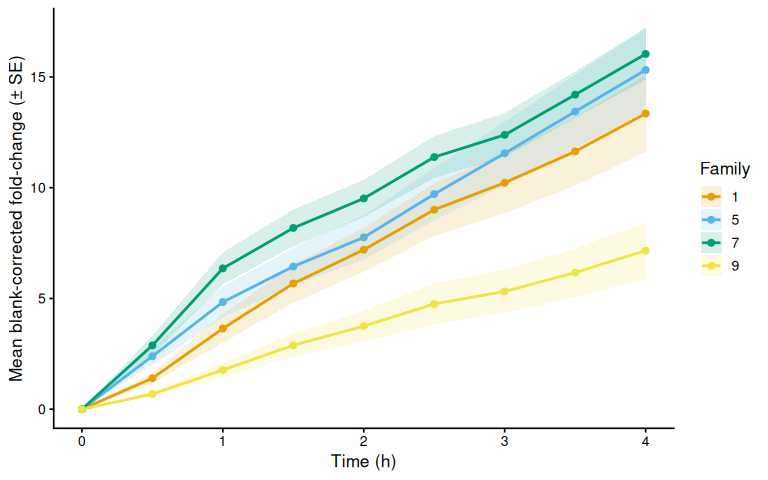

ggsave(file.path(fig_dir, "blank_corrected_fc_mean_by_family.png"),
       p_bc_fc_mean, width = 8, height = 5)

8.2 Individual traces by family

p_bc_fc_by_family <- samples %>%
  filter(!is.na(family_id_group)) %>%
  ggplot(aes(x = time_hr, y = corrected_fc, group = trace_id,
             colour = .data[[if (has_trt) "treatment_group" else "family_id_group"]])) +
  geom_line(alpha = 0.6) +
  geom_point(size = 1.2, alpha = 0.7) +
  facet_wrap(~ family_id_group) +
  scale_colour_manual(
    values = if (has_trt) trt_colours else fam_colours,
    name   = if (has_trt) "Treatment" else "Family",
    breaks = if (has_trt) treatments else families) +
  labs(x = "Time (h)", y = "Blank-corrected fold-change") +
  theme_classic(base_size = 12) +
  theme(strip.background = element_blank(),
        strip.text       = element_text(face = "bold"))

p_bc_fc_by_family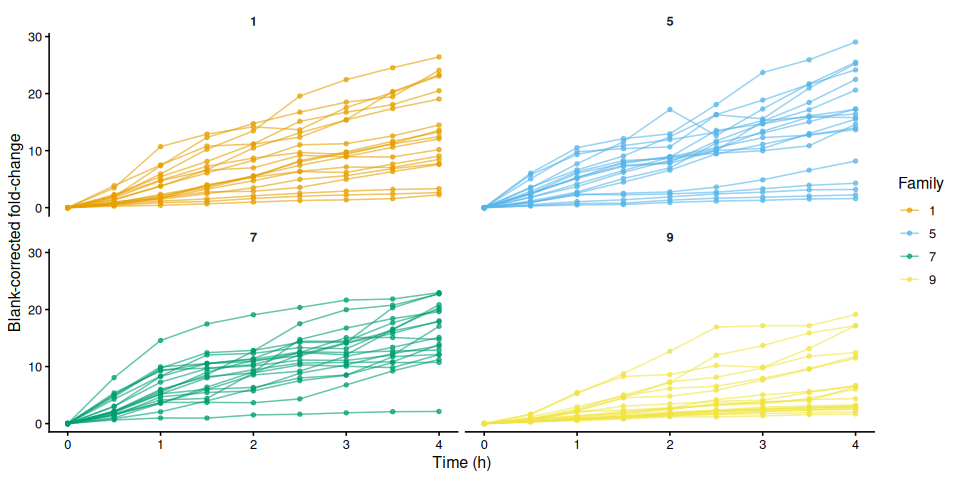

ggsave(file.path(fig_dir, "blank_corrected_fc_by_family.png"),
       p_bc_fc_by_family, width = 10, height = 5)

8.3 Individual blank-corrected fold-change traces by treatment

if (has_trt) {
  p_bc_fc_by_treatment <- samples %>%
    ggplot(aes(x = time_hr, y = corrected_fc,
               group = trace_id, colour = family_id_group)) +
    geom_line(alpha = 0.6) +
    geom_point(size = 1.2, alpha = 0.7) +
    facet_wrap(~ treatment_group) +
    scale_colour_manual(values = fam_colours, name = "Family",
                        breaks = families) +
    labs(x = "Time (h)", y = "Blank-corrected fold-change") +
    theme_classic(base_size = 12) +
    theme(strip.background = element_blank(),
          strip.text       = element_text(face = "bold"))

  p_bc_fc_by_treatment
  ggsave(file.path(fig_dir, "blank_corrected_fc_by_treatment.png"),
         p_bc_fc_by_treatment, width = 10, height = 5)
}

9 Metabolism (Size-Normalised Fold-Change)

Blank-corrected fold-change divided by each active measurement column. This is “metabolism” as defined in Huffmyer et al.

if (length(active_meas_cols) == 0) {
  message("No active measurement columns: skipping metabolism calculation.")
  metabolism_df <- tibble()
} else {
  metabolism_df <- samples
  for (mc in active_meas_cols) {
    out_col <- paste0("metabolism_per_", mc)
    metabolism_df <- metabolism_df %>%
      mutate(!!out_col := if_else(
        is.finite(.data[[mc]]) & .data[[mc]] > 0 &
          is.finite(corrected_fc),
        corrected_fc / .data[[mc]],
        NA_real_
      ))
  }
}

str(metabolism_df)

tibble [1,191 × 24] (S3: tbl_df/tbl/data.frame)
 $ row_id                             : chr [1:1191] "A" "A" "A" "A" ...
 $ col_id                             : int [1:1191] 1 2 3 4 5 6 7 8 9 10 ...
 $ well_id                            : chr [1:1191] "A1" "A2" "A3" "A4" ...
 $ value                              : num [1:1191] 596 597 605 613 601 626 626 626 610 636 ...
 $ plate_id                           : chr [1:1191] "a" "a" "a" "a" ...
 $ time_hr                            : num [1:1191] 0 0 0 0 0 0 0 0 0 0 ...
 $ is_blank                           : logi [1:1191] FALSE FALSE FALSE FALSE FALSE FALSE ...
 $ exclude_from_analysis              : logi [1:1191] FALSE FALSE FALSE FALSE FALSE FALSE ...
 $ exclude_reason                     : chr [1:1191] NA NA NA NA ...
 $ family_id_group                    : chr [1:1191] "7" "5" "1" "9" ...
 $ sample_id_group                    : chr [1:1191] "1" "2" "3" "4" ...
 $ treatment_group                    : chr [1:1191] NA NA NA NA ...
 $ width_mm_measurement               : num [1:1191] NA NA NA NA NA NA NA NA NA NA ...
 $ length_mm_measurement              : num [1:1191] NA NA NA NA NA NA NA NA NA NA ...
 $ weight_mg_measurement              : num [1:1191] NA NA NA NA NA NA NA NA NA NA ...
 $ area_mm2_measurement               : num [1:1191] 538 586 713 757 823 ...
 $ sample_key                         : chr [1:1191] "1" "2" "3" "4" ...
 $ value_t0                           : num [1:1191] 596 597 605 613 601 626 626 626 610 636 ...
 $ fold_change                        : num [1:1191] 1 1 1 1 1 1 1 1 1 1 ...
 $ trace_id                           : chr [1:1191] "1" "2" "3" "4" ...
 $ mean_blank_rfu                     : num [1:1191] 663 663 663 663 663 ...
 $ mean_blank_fc                      : num [1:1191] 1 1 1 1 1 1 1 1 1 1 ...
 $ corrected_fc                       : num [1:1191] 0 0 0 0 0 0 0 0 0 0 ...
 $ metabolism_per_area_mm2_measurement: num [1:1191] 0 0 0 0 0 0 0 0 0 0 ...

9.1 Mean metabolism by family

if (nrow(metabolism_df) > 0) {

  metab_cols <- paste0("metabolism_per_", active_meas_cols)

  for (col in metab_cols) {
    if (!col %in% names(metabolism_df)) next
    mc_label <- str_remove(col, "^metabolism_per_")

    metab_summary <- metabolism_df %>%
      filter(!is.na(family_id_group), !exclude_from_analysis) %>%
      group_by(family_id_group, treatment_group, time_hr) %>%
      summarise(
        mean_val = mean(.data[[col]], na.rm = TRUE),
        se_val   = sd(.data[[col]], na.rm = TRUE) /
          sqrt(sum(!is.na(.data[[col]]))),
        .groups  = "drop"
      ) %>%
      mutate(group_var = if (has_trt)
        paste(family_id_group, treatment_group, sep = ".")
      else
        family_id_group)

    p_metab_mean <- ggplot(metab_summary,
        aes(x = time_hr, y = mean_val,
            colour = family_id_group,
            group = group_var)) +
      geom_ribbon(aes(ymin = mean_val - se_val,
                      ymax = mean_val + se_val,
                      fill = family_id_group),
                  alpha = 0.15, colour = NA) +
      geom_line(
        mapping   = if (has_trt) aes(linetype = treatment_group) else NULL,
        linewidth = 1) +
      geom_point(size = 2) +
      scale_colour_manual(values = fam_colours, name = "Family",
                          breaks = families) +
      scale_fill_manual(values = fam_colours, name = "Family",
                        breaks = families) +
      labs(x = "Time (h)",
           y = paste0(metabolism_y_label(col), " (± SE)")) +
      theme_classic(base_size = 13) +
      if (has_trt) scale_linetype_manual(values = trt_linetypes, name = "Treatment") else NULL

    print(p_metab_mean)
    ggsave(
      file.path(fig_dir,
                paste0("metabolism_mean_", mc_label, ".png")),
      p_metab_mean, width = 8, height = 5)
  }
}

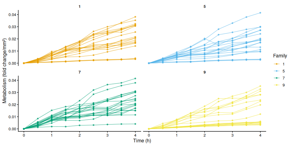
9.2 Individual metabolism traces by family

if (nrow(metabolism_df) > 0) {

  for (col in metab_cols) {
    if (!col %in% names(metabolism_df)) next
    mc_label <- str_remove(col, "^metabolism_per_")

    p_metab_by_family <- metabolism_df %>%
      filter(!is.na(family_id_group)) %>%
      ggplot(aes(x = time_hr, y = .data[[col]], group = trace_id,
                 colour = .data[[if (has_trt) "treatment_group" else "family_id_group"]])) +
      geom_line(alpha = 0.6) +
      geom_point(size = 1.2, alpha = 0.7) +
      facet_wrap(~ family_id_group) +
      scale_colour_manual(
        values = if (has_trt) trt_colours else fam_colours,
        name   = if (has_trt) "Treatment" else "Family",
        breaks = if (has_trt) treatments else families) +
      labs(x = "Time (h)", y = metabolism_y_label(col)) +
      theme_classic(base_size = 12) +
      theme(strip.background = element_blank(),
            strip.text       = element_text(face = "bold"))

    print(p_metab_by_family)
    ggsave(
      file.path(fig_dir,
                paste0("metabolism_individual_", mc_label, "_by_family.png")),
      p_metab_by_family, width = 10, height = 5)

    if (has_trt) {
      p_metab_by_treatment <- ggplot(metabolism_df,
          aes(x = time_hr, y = .data[[col]],
              group = trace_id, colour = family_id_group)) +
        geom_line(alpha = 0.6) +
        geom_point(size = 1.2, alpha = 0.7) +
        facet_wrap(~ treatment_group) +
        scale_colour_manual(values = fam_colours, name = "Family",
                            breaks = families) +
        labs(x = "Time (h)", y = metabolism_y_label(col)) +
        theme_classic(base_size = 12) +
        theme(strip.background = element_blank(),
              strip.text       = element_text(face = "bold"))

      print(p_metab_by_treatment)
      ggsave(
        file.path(fig_dir,
                  paste0("metabolism_individual_", mc_label, "_by_treatment.png")),
        p_metab_by_treatment, width = 10, height = 5)
    }
  }
}

10 Time-Series Statistical Analysis

Linear mixed effects models test the effect of experimental variables on metabolism over time. Individual (sample_id_group) is included as a random intercept to account for repeated measures across timepoints. Type III ANOVA with Satterthwaite’s approximation (lmerTest) assesses significance; post-hoc pairwise comparisons use estimated marginal means (emmeans, Tukey adjustment).

run_ts_stats <- function(df, value_col) {
  has_family    <- "family_id_group" %in% names(df) &&
    length(unique(na.omit(df$family_id_group))) > 1
  has_treatment <- "treatment_group" %in% names(df) &&
    length(unique(na.omit(df$treatment_group))) > 1

  if (!has_family && !has_treatment) return(NULL)

  df <- df %>%
    filter(is.finite(.data[[value_col]]), is.finite(time_hr)) %>%
    mutate(
      time_f     = factor(time_hr),
      individual = factor(trace_id)
    )

  if (nrow(df) == 0) return(NULL)

  if (has_family)    df <- df %>% mutate(family    = factor(family_id_group))
  if (has_treatment) df <- df %>% mutate(treatment = factor(treatment_group))

  if (has_family    && length(unique(na.omit(df$family)))    < 2) return(NULL)
  if (has_treatment && length(unique(na.omit(df$treatment))) < 2) return(NULL)

  fixed <- if (has_family && has_treatment) {
    paste0(value_col, " ~ time_f * family * treatment")
  } else if (has_family) {
    paste0(value_col, " ~ time_f * family")
  } else {
    paste0(value_col, " ~ time_f * treatment")
  }

  model <- lmer(
    as.formula(paste0(fixed, " + (1 | individual)")),
    data = df
  )

  anova_res <- anova(model, type = 3, ddf = "Satterthwaite")

  # Pairwise comparisons of group combinations at each timepoint
  emm_spec <- if (has_family && has_treatment) {
    ~ family * treatment | time_f
  } else if (has_family) {
    ~ family | time_f
  } else {
    ~ treatment | time_f
  }

  emm       <- emmeans(model, emm_spec)
  pairs_res <- as.data.frame(pairs(emm, adjust = "tukey"))

  # Main-effect marginal means (collapsed across time)
  emm_main <- if (has_family && has_treatment) {
    emmeans(model, ~ family * treatment)
  } else if (has_family) {
    emmeans(model, ~ family)
  } else {
    emmeans(model, ~ treatment)
  }

  pairs_main <- as.data.frame(pairs(emm_main, adjust = "tukey"))

  list(
    model         = model,
    anova         = anova_res,
    pairs_by_time = pairs_res,
    pairs_main    = pairs_main,
    has_family    = has_family,
    has_treatment = has_treatment
  )
}

ts_stats <- list()
if (nrow(metabolism_df) > 0) {
  for (mc in active_meas_cols) {
    col <- paste0("metabolism_per_", mc)
    if (col %in% names(metabolism_df))
      ts_stats[[col]] <- run_ts_stats(metabolism_df, col)
  }
}

10.1 Results

for (col in names(ts_stats)) {
  res <- ts_stats[[col]]
  if (is.null(res)) next

  cat("\n\n### Metric:", col, "\n\n")

  cat("**Type III ANOVA (Satterthwaite approximation):**\n\n")
  cat(knitr::kable(as.data.frame(res$anova), digits = 4, format = "pipe"), sep = "\n")
  cat("\n")

  cat("**Marginal means – main effects (collapsed across time):**\n\n")
  cat(knitr::kable(as.data.frame(res$pairs_main), digits = 4, format = "pipe"), sep = "\n")
  cat("\n")

  cat("**Pairwise comparisons by timepoint (Tukey):**\n\n")
  cat(knitr::kable(as.data.frame(res$pairs_by_time), digits = 4, format = "pipe"), sep = "\n")
  cat("\n")
}

10.1.1 Metric: metabolism_per_area_mm2_measurement

Type III ANOVA (Satterthwaite approximation):

	Sum Sq	Mean Sq	NumDF	DenDF	F value	Pr(>F)
time_f	0.0269	0.0034	8	592	201.3951	0.0000
family	0.0002	0.0001	3	74	4.1895	0.0085
time_f:family	0.0009	0.0000	24	592	2.2689	0.0006

Marginal means – main effects (collapsed across time):

contrast	estimate	SE	df	t.ratio	p.value
family1 - family5	0.0018	0.0017	74	1.0878	0.6980
family1 - family7	-0.0015	0.0017	74	-0.9143	0.7973
family1 - family9	0.0040	0.0017	74	2.4052	0.0849
family5 - family7	-0.0033	0.0017	74	-2.0160	0.1914
family5 - family9	0.0022	0.0017	74	1.3035	0.5636
family7 - family9	0.0055	0.0016	74	3.3629	0.0066

Pairwise comparisons by timepoint (Tukey):

contrast	time_f	estimate	SE	df	t.ratio	p.value
family1 - family5	0	0.0000	0.0021	172.1828	0.0000	1.0000
family1 - family7	0	0.0000	0.0021	172.1828	0.0000	1.0000
family1 - family9	0	0.0000	0.0021	172.1828	0.0000	1.0000
family5 - family7	0	0.0000	0.0021	172.1828	0.0000	1.0000
family5 - family9	0	0.0000	0.0021	172.1828	0.0000	1.0000
family7 - family9	0	0.0000	0.0020	172.1828	0.0000	1.0000
family1 - family5	0.5	-0.0004	0.0021	172.1828	-0.1799	0.9979
family1 - family7	0.5	-0.0015	0.0021	172.1828	-0.7412	0.8803
family1 - family9	0.5	0.0007	0.0021	172.1828	0.3484	0.9854
family5 - family7	0.5	-0.0012	0.0021	172.1828	-0.5591	0.9440
family5 - family9	0.5	0.0011	0.0021	172.1828	0.5306	0.9515
family7 - family9	0.5	0.0023	0.0020	172.1828	1.1039	0.6876
family1 - family5	1	0.0001	0.0021	172.1828	0.0474	1.0000
family1 - family7	1	-0.0029	0.0021	172.1828	-1.4243	0.4860
family1 - family9	1	0.0019	0.0021	172.1828	0.9313	0.7881
family5 - family7	1	-0.0030	0.0021	172.1828	-1.4723	0.4565
family5 - family9	1	0.0018	0.0021	172.1828	0.8833	0.8135
family7 - family9	1	0.0049	0.0020	172.1828	2.3864	0.0835
family1 - family5	1.5	0.0014	0.0021	172.1828	0.6526	0.9145
family1 - family7	1.5	-0.0023	0.0021	172.1828	-1.1083	0.6849
family1 - family9	1.5	0.0030	0.0021	172.1828	1.4675	0.4594
family5 - family7	1.5	-0.0037	0.0021	172.1828	-1.7692	0.2917
family5 - family9	1.5	0.0017	0.0021	172.1828	0.8066	0.8512
family7 - family9	1.5	0.0053	0.0020	172.1828	2.6095	0.0481
family1 - family5	2	0.0023	0.0021	172.1828	1.0860	0.6985
family1 - family7	2	-0.0018	0.0021	172.1828	-0.8513	0.8297
family1 - family9	2	0.0041	0.0021	172.1828	1.9992	0.1923
family5 - family7	2	-0.0040	0.0021	172.1828	-1.9512	0.2108
family5 - family9	2	0.0019	0.0021	172.1828	0.8994	0.8052
family7 - family9	2	0.0059	0.0020	172.1828	2.8878	0.0225
family1 - family5	2.5	0.0032	0.0021	172.1828	1.5385	0.4168
family1 - family7	2.5	-0.0013	0.0021	172.1828	-0.6306	0.9221
family1 - family9	2.5	0.0056	0.0021	172.1828	2.7107	0.0368
family5 - family7	2.5	-0.0045	0.0021	172.1828	-2.1887	0.1305
family5 - family9	2.5	0.0024	0.0021	172.1828	1.1526	0.6575
family7 - family9	2.5	0.0069	0.0020	172.1828	3.3850	0.0048
family1 - family5	3	0.0031	0.0021	172.1828	1.4628	0.4623
family1 - family7	3	-0.0011	0.0021	172.1828	-0.5329	0.9510
family1 - family9	3	0.0062	0.0021	172.1828	3.0222	0.0152
family5 - family7	3	-0.0042	0.0021	172.1828	-2.0143	0.1867
family5 - family9	3	0.0032	0.0021	172.1828	1.5408	0.4155
family7 - family9	3	0.0073	0.0020	172.1828	3.6016	0.0023
family1 - family5	3.5	0.0031	0.0021	172.1828	1.4823	0.4504
family1 - family7	3.5	-0.0015	0.0021	172.1828	-0.7074	0.8940
family1 - family9	3.5	0.0067	0.0021	172.1828	3.2489	0.0075
family5 - family7	3.5	-0.0046	0.0021	172.1828	-2.2086	0.1250
family5 - family9	3.5	0.0036	0.0021	172.1828	1.7477	0.3024
family7 - family9	3.5	0.0082	0.0020	172.1828	4.0080	0.0005
family1 - family5	4	0.0037	0.0021	172.1828	1.7631	0.2948
family1 - family7	4	-0.0012	0.0021	172.1828	-0.6040	0.9307
family1 - family9	4	0.0075	0.0021	172.1828	3.6345	0.0021
family5 - family7	4	-0.0049	0.0021	172.1828	-2.3895	0.0829
family5 - family9	4	0.0038	0.0021	172.1828	1.8489	0.2542
family7 - family9	4	0.0088	0.0020	172.1828	4.2938	0.0002

11 Area Under the Curve (AUC)

AUC computed per individual via the trapezoid rule across all timepoints. metabolism_per_* is the primary metric matching the paper; corrected_fc and raw_fluorescence are retained for reference.

compute_auc <- function(df, value_col, group_vars) {
  df %>%
    filter(is.finite(time_hr), is.finite(.data[[value_col]])) %>%
    group_by(across(all_of(group_vars))) %>%
    summarise(
      AUC          = trapezoid_auc(time_hr, .data[[value_col]]),
      n_timepoints = n(),
      .groups      = "drop"
    ) %>%
    filter(is.finite(AUC))
}

# Only include grouping columns that are actually present in the data
individual_vars <- intersect(
  c("trace_id", "family_id_group", "treatment_group"),
  names(metabolism_df)
)

auc_metab_list <- list()
if (nrow(metabolism_df) > 0) {
  for (mc in active_meas_cols) {
    col <- paste0("metabolism_per_", mc)
    if (col %in% names(metabolism_df)) {
      auc_metab_list[[col]] <-
        compute_auc(metabolism_df, col, individual_vars) %>%
        mutate(metric = col)
    }
  }
}

auc_all <- bind_rows(auc_metab_list)

str(auc_all)

tibble [78 × 6] (S3: tbl_df/tbl/data.frame)
 $ trace_id       : chr [1:78] "1" "10" "11" "12" ...
 $ family_id_group: chr [1:78] "7" "5" "1" "9" ...
 $ treatment_group: chr [1:78] NA NA NA NA ...
 $ AUC            : num [1:78] 0.0359 0.0813 0.0489 0.0122 0.0505 ...
 $ n_timepoints   : int [1:78] 9 9 9 9 9 9 9 9 9 9 ...
 $ metric         : chr [1:78] "metabolism_per_area_mm2_measurement" "metabolism_per_area_mm2_measurement" "metabolism_per_area_mm2_measurement" "metabolism_per_area_mm2_measurement" ...

11.1 AUC summary tables

sum_vars <- intersect(
  c("metric", "family_id_group", "treatment_group"),
  names(auc_all)
)
auc_summary <- auc_all %>%
  group_by(across(all_of(sum_vars))) %>%
  summarise(
    n      = n(),
    mean   = mean(AUC, na.rm = TRUE),
    sd     = sd(AUC, na.rm = TRUE),
    se     = sd / sqrt(n),
    median = median(AUC, na.rm = TRUE),
    .groups = "drop"
  )

print(auc_summary)

# A tibble: 4 × 8
  metric      family_id_group treatment_group     n   mean     sd      se median
  <chr>       <chr>           <chr>           <int>  <dbl>  <dbl>   <dbl>  <dbl>
1 metabolism… 1               <NA>               19 0.0446 0.0215 0.00493 0.0441
2 metabolism… 5               <NA>               19 0.0373 0.0204 0.00467 0.0366
3 metabolism… 7               <NA>               20 0.0511 0.0179 0.00400 0.0513
4 metabolism… 9               <NA>               20 0.0285 0.0228 0.00510 0.0124

12 Statistical Analysis

Each individual oyster (sample_id_group) is the observational unit. The model is built from whichever grouping factors are present: both family and treatment (with interaction) when both exist, or a one-way model when only one factor is available. Each plate maps to a unique family × treatment combination, so plate-level and group-level variance are confounded; interpret accordingly.

run_auc_stats <- function(auc_df) {
  empty <- tibble()

  has_family    <- "family_id_group" %in% names(auc_df) &&
    length(unique(na.omit(auc_df$family_id_group))) > 1
  has_treatment <- "treatment_group" %in% names(auc_df) &&
    length(unique(na.omit(auc_df$treatment_group))) > 1

  if (!has_family && !has_treatment) {
    return(list(model = NULL, anova = NULL,
                pairs_full = empty, pairs_family = empty,
                pairs_trt = empty,
                has_family = FALSE, has_treatment = FALSE))
  }

  if (has_family)    auc_df <- auc_df %>% mutate(family    = factor(family_id_group))
  if (has_treatment) auc_df <- auc_df %>% mutate(treatment = factor(treatment_group))

  formula_str <- if (has_family && has_treatment) {
    "AUC ~ family * treatment"
  } else if (has_family) {
    "AUC ~ family"
  } else {
    "AUC ~ treatment"
  }
  model     <- lm(as.formula(formula_str), data = auc_df)
  anova_res <- anova(model)

  if (has_family && has_treatment) {
    pairs_full   <- as.data.frame(pairs(emmeans(model, ~ family * treatment),
                                        adjust = "tukey"))
    pairs_family <- as.data.frame(pairs(emmeans(model, ~ family),
                                        adjust = "tukey"))
    pairs_trt    <- as.data.frame(pairs(emmeans(model, ~ treatment),
                                        adjust = "tukey"))
  } else if (has_family) {
    pairs_family <- as.data.frame(pairs(emmeans(model, ~ family),
                                        adjust = "tukey"))
    pairs_full   <- pairs_family
    pairs_trt    <- empty
  } else {
    pairs_trt    <- as.data.frame(pairs(emmeans(model, ~ treatment),
                                        adjust = "tukey"))
    pairs_full   <- pairs_trt
    pairs_family <- empty
  }

  list(
    model         = model,
    anova         = anova_res,
    pairs_full    = pairs_full,
    pairs_family  = pairs_family,
    pairs_trt     = pairs_trt,
    has_family    = has_family,
    has_treatment = has_treatment
  )
}

metrics_to_test <- unique(auc_all$metric)
stats_results   <- map(
  set_names(metrics_to_test),
  ~ run_auc_stats(auc_all %>% filter(metric == .x))
)

12.1 Results by metric

for (met in metrics_to_test) {
  stats <- stats_results[[met]]
  cat("\n\n### Metric:", met, "\n\n")
  cat("**ANOVA:**\n\n")
  cat(knitr::kable(as.data.frame(stats$anova), digits = 4, format = "pipe"), sep = "\n")
  cat("\n")
  if (stats$has_family && stats$has_treatment) {
    cat("**Pairwise: family × treatment (Tukey):**\n\n")
    cat(knitr::kable(as.data.frame(stats$pairs_full), digits = 4, format = "pipe"), sep = "\n")
  cat("\n")
    cat("**Pairwise: family main effect:**\n\n")
    cat(knitr::kable(as.data.frame(stats$pairs_family), digits = 4, format = "pipe"), sep = "\n")
  cat("\n")
    cat("**Pairwise: treatment main effect:**\n\n")
    cat(knitr::kable(as.data.frame(stats$pairs_trt), digits = 4, format = "pipe"), sep = "\n")
  cat("\n")
  } else if (stats$has_family) {
    cat("**Pairwise: family (Tukey):**\n\n")
    cat(knitr::kable(as.data.frame(stats$pairs_family), digits = 4, format = "pipe"), sep = "\n")
  cat("\n")
  } else if (stats$has_treatment) {
    cat("**Pairwise: treatment (Tukey):**\n\n")
    cat(knitr::kable(as.data.frame(stats$pairs_trt), digits = 4, format = "pipe"), sep = "\n")
  cat("\n")
  }
}

12.1.1 Metric: metabolism_per_area_mm2_measurement

ANOVA:

	Df	Sum Sq	Mean Sq	F value	Pr(>F)
family	3	0.0056	0.0019	4.3721	0.0069
Residuals	74	0.0317	0.0004	NA	NA

Pairwise: family (Tukey):

contrast	estimate	SE	df	t.ratio	p.value
family1 - family5	0.0073	0.0067	74	1.0858	0.6993
family1 - family7	-0.0065	0.0066	74	-0.9809	0.7607
family1 - family9	0.0161	0.0066	74	2.4212	0.0819
family5 - family7	-0.0138	0.0066	74	-2.0806	0.1690
family5 - family9	0.0088	0.0066	74	1.3216	0.5523
family7 - family9	0.0226	0.0065	74	3.4467	0.0051

13 AUC Box Plots with Statistical Annotations

Significance labels: *** p < 0.001, ** p < 0.01, * p < 0.05. Brackets are drawn only for significant pairs (p < 0.05). Plots are generated for whichever grouping factors are present: treatment-only, family-only, all-groups, within-family, and within-treatment.

sig_label <- function(p) {
  case_when(p < 0.001 ~ "***", p < 0.01 ~ "**", p < 0.05 ~ "*",
            TRUE ~ "ns")
}

# Add significance brackets to an existing ggplot.
# pairs_df   : data frame with $contrast and $p.value columns
# group_levels: ordered character vector matching x-axis factor levels
# y_vals     : numeric vector of AUC values used to set bracket heights
add_sig_brackets <- function(p, pairs_df, group_levels, y_vals) {
  sig_pairs <- pairs_df %>%
    mutate(label = sig_label(p.value)) %>%
    filter(label != "ns")
  if (nrow(sig_pairs) == 0) return(p)

  y_max   <- max(y_vals, na.rm = TRUE)
  y_range <- diff(range(y_vals, na.rm = TRUE))
  step    <- y_range * 0.12

  # emmeans prefixes factor levels with the variable name (e.g. "family7");
  # resolve back to the bare level used on the x-axis.
  resolve_level <- function(x, lvls) {
    x <- trimws(x)
    if (x %in% lvls) return(x)
    lvls_sorted <- lvls[order(nchar(as.character(lvls)), decreasing = TRUE)]
    for (lvl in lvls_sorted) {
      lvl_str <- as.character(lvl)
      if (endsWith(x, lvl_str) && nchar(x) > nchar(lvl_str)) return(lvl_str)
    }
    NA_character_
  }

  for (i in seq_len(nrow(sig_pairs))) {
    parts <- str_split(as.character(sig_pairs$contrast[i]), " - ", 2)[[1]]
    g1 <- resolve_level(parts[1], group_levels)
    g2 <- resolve_level(parts[2], group_levels)
    x1 <- match(g1, group_levels)
    x2 <- match(g2, group_levels)
    if (is.na(x1) || is.na(x2)) next
    bar_y <- y_max + i * step
    p <- p +
      annotate("segment", x = x1, xend = x2,
               y = bar_y, yend = bar_y,
               colour = "black", linewidth = 0.6) +
      annotate("segment", x = x1, xend = x1,
               y = bar_y, yend = bar_y - step * 0.3,
               colour = "black", linewidth = 0.6) +
      annotate("segment", x = x2, xend = x2,
               y = bar_y, yend = bar_y - step * 0.3,
               colour = "black", linewidth = 0.6) +
      annotate("text", x = (x1 + x2) / 2,
               y = bar_y + step * 0.15,
               label = sig_pairs$label[i], size = 4.5)
  }
  p
}

for (met in metrics_to_test) {
  df      <- auc_all %>% filter(metric == met)
  stats   <- stats_results[[met]]
  y_lab   <- auc_y_label(met)
  has_fam <- stats$has_family
  has_trt <- stats$has_treatment

  # ── Treatment main effect (x = treatment, tick = treatment name) ───────
  if (has_trt) {
    df_p <- df %>%
      mutate(x = factor(treatment_group, levels = sort(unique(treatment_group))))
    grps <- levels(df_p$x)
    p <- ggplot(df_p, aes(x = x, y = AUC, fill = x)) +
      geom_boxplot(alpha = 0.6, outlier.shape = NA) +
      geom_jitter(width = 0.15, alpha = 0.4, size = 1.5) +
      scale_fill_manual(values = trt_colours[grps], guide = "none") +
      labs(x = "Treatment", y = y_lab) +
      theme_classic(base_size = 13)
    p <- add_sig_brackets(p, stats$pairs_trt, grps, df_p$AUC)
    print(p)
    ggsave(file.path(fig_dir, paste0("auc_treatment_", met, ".png")),
           p, width = 5, height = 5)
  }

  # ── Family main effect (x = family, tick = family name) ───────────────
  if (has_fam) {
    df_p <- df %>%
      mutate(x = factor(family_id_group,
                        levels = str_sort(unique(family_id_group), numeric = TRUE)))
    grps <- levels(df_p$x)
    p <- ggplot(df_p, aes(x = x, y = AUC, fill = x)) +
      geom_boxplot(alpha = 0.6, outlier.shape = NA) +
      geom_jitter(width = 0.15, alpha = 0.4, size = 1.5) +
      scale_fill_manual(values = fam_colours[grps], guide = "none") +
      labs(x = "Family", y = y_lab) +
      theme_classic(base_size = 13)
    p <- add_sig_brackets(p, stats$pairs_family, grps, df_p$AUC)
    print(p)
    ggsave(file.path(fig_dir, paste0("auc_family_", met, ".png")),
           p, width = 5, height = 5)
  }

  # Remaining plots require both factors
  if (!has_fam || !has_trt) next

  # ── All family:treatment groups (x = family:treatment) ─────────────────
  # emmeans contrasts use spaces; convert to colon to match tick labels
  pairs_fc <- stats$pairs_full %>%
    mutate(contrast = str_replace_all(
      contrast,
      "([a-z]+) ([a-z]+)( - )([a-z]+) ([a-z]+)",
      "\\1:\\2\\3\\4:\\5"
    ))
  df_p <- df %>%
    mutate(x = factor(
      paste(family_id_group, treatment_group, sep = ":"),
      levels = str_sort(unique(paste(family_id_group, treatment_group, sep = ":")),
                        numeric = TRUE)
    ))
  grps     <- levels(df_p$x)
  fill_map <- setNames(make_palette(length(grps)), grps)
  p <- ggplot(df_p, aes(x = x, y = AUC, fill = x)) +
    geom_boxplot(alpha = 0.6, outlier.shape = NA) +
    geom_jitter(width = 0.15, alpha = 0.4, size = 1.5) +
    scale_fill_manual(values = fill_map, guide = "none") +
    labs(x = "Family : Treatment", y = y_lab) +
    theme_classic(base_size = 13) +
    theme(axis.text.x = element_text(angle = 20, hjust = 1))
  p <- add_sig_brackets(p, pairs_fc, grps, df_p$AUC)
  print(p)
  ggsave(file.path(fig_dir, paste0("auc_all_groups_", met, ".png")),
         p, width = 6, height = 5)

  # ── Within each family: treatment comparison (x = family:treatment) ────
  # Tick labels are family:treatment so these plots are visually distinct
  # from the treatment main-effect plot above.
  for (fam in str_sort(unique(df$family_id_group), numeric = TRUE)) {
    df_p <- df %>%
      filter(family_id_group == fam) %>%
      mutate(x = factor(
        paste(family_id_group, treatment_group, sep = ":"),
        levels = str_sort(unique(paste(family_id_group, treatment_group, sep = ":")),
                          numeric = TRUE)
      ))
    grps     <- levels(df_p$x)
    pairs_sub <- pairs_fc %>%
      filter(str_count(contrast, paste0(fam, ":")) == 2)
    p <- ggplot(df_p, aes(x = x, y = AUC, fill = x)) +
      geom_boxplot(alpha = 0.6, outlier.shape = NA) +
      geom_jitter(width = 0.15, alpha = 0.4, size = 1.5) +
      scale_fill_manual(values = fill_map[grps], guide = "none") +
      labs(x = "Family : Treatment", y = y_lab) +
      theme_classic(base_size = 13)
    p <- add_sig_brackets(p, pairs_sub, grps, df_p$AUC)
    print(p)
    ggsave(file.path(fig_dir, paste0("auc_", fam, "_trt_", met, ".png")),
           p, width = 5, height = 5)
  }

  # ── Within each treatment: family comparison (x = family:treatment) ────
  # Tick labels are family:treatment so these plots are visually distinct
  # from the family main-effect plot above.
  for (trt in sort(unique(df$treatment_group))) {
    df_p <- df %>%
      filter(treatment_group == trt) %>%
      mutate(x = factor(
        paste(family_id_group, treatment_group, sep = ":"),
        levels = str_sort(unique(paste(family_id_group, treatment_group, sep = ":")),
                          numeric = TRUE)
      ))
    grps      <- levels(df_p$x)
    pairs_sub <- pairs_fc %>%
      filter(str_count(contrast, paste0(":", trt)) == 2)
    p <- ggplot(df_p, aes(x = x, y = AUC, fill = x)) +
      geom_boxplot(alpha = 0.6, outlier.shape = NA) +
      geom_jitter(width = 0.15, alpha = 0.4, size = 1.5) +
      scale_fill_manual(values = fill_map[grps], guide = "none") +
      labs(x = "Family : Treatment", y = y_lab) +
      theme_classic(base_size = 13)
    p <- add_sig_brackets(p, pairs_sub, grps, df_p$AUC)
    print(p)
    ggsave(file.path(fig_dir, paste0("auc_", trt, "_fam_", met, ".png")),
           p, width = 5, height = 5)
  }
}

14 Save Output Data

write_csv(auc_all,      file.path(out_dir, "auc_all_metrics.csv"))
write_csv(auc_summary,  file.path(out_dir, "auc_summary.csv"))

if (nrow(metabolism_df) > 0)
  write_csv(metabolism_df,
            file.path(out_dir, "metabolism.csv"))

stats_compiled <- map_dfr(metrics_to_test, function(met) {
  bind_rows(
    stats_results[[met]]$pairs_full %>%
      mutate(comparison = "family:treatment"),
    stats_results[[met]]$pairs_family %>%
      mutate(comparison = "family"),
    stats_results[[met]]$pairs_trt %>%
      mutate(comparison = "treatment")
  ) %>% mutate(metric = met)
})

write_csv(stats_compiled,
          file.path(out_dir, "pairwise_stats.csv"))

message("Output files written to: ", out_dir)