Citrate Synthase Assay - SORMI June 2026 M.gigas Family 5 Ambient Ctenidia Re-assay

INTRO

This is a re-assay of the eight Magallana gigas (Pacific oyster) Family 5 ctenidia homogenates held at ambient temperature, using the Citrate Synthase Assay Kit (ABCAM; cat: ab239712). The original assay of these same homogenates on 20260811 (Notebook entry) had QC failures serious enough that its activity values could not be used — a failed GSH standard curve, standards above the photometric linear range, background control wells behaving as active reactions, and one sample (F05_05_ambient) with no clean replicate. This plate is the re-run called for by that entry.

Two things changed relative to the 20260811 run: a shorter read window (20 min / 11 reads, vs. 40 min / 21 reads) and a pooled background control design in place of paired per-sample backgrounds. Samples had been previously homogenized on 20260811 (Notebook entry), and protein concentrations for normalization were determined on 20260813 (Notebook entry) — the same homogenates and the same protein measurements used for the original assay.

Note

This re-assay succeeded and supersedes the 20260811 ambient results. No sample well, positive-control well, or background well is flagged for anything on this plate: no decreasing kinetics, no read glitches, no elevated starting absorbance, and all three pooled-background replicates are flat. All eight samples pass the 15% technical CV threshold (0.8-4.6%), the GSH standard curve has zero flagged outlier wells (R² = 0.9983), and no replicate is excluded from any sample. This plate does not need re-assay.

One caution worth carrying forward: the positive control’s three replicates rise linearly (R² 0.997-1.000) but disagree in rate by 22.8% CV (D7 at 2.00 mA412/min vs. D8/D9 at 2.95-3.15 mA412/min) — worse precision than any individual sample’s technical triplicate on this plate. This does not enter any activity calculation, so it is a plate-level caution rather than a disqualifier, but it is worth watching on future plates.

All data/code/analysis is available here:

• https://github.com/RobertsLab/sormi-assay-development/tree/main/Citrate_synthase

MATERIALS & METHODS

Citrate Synthase Assay

The Citrate Synthase Assay Kit (ABCAM; cat: ab239712) was used according to the manufacturer’s instructions (ABCAM-Citrate-Synthase-Assay-v4a-ab239712.pdf (GitHub; PDF)). The kit is a coupled kinetic assay: citrate synthase condenses acetyl-CoA and oxaloacetate to release free CoA-SH, the liberated thiol reduces DTNB to TNB^2-, and the rate of absorbance increase at 412 nm is proportional to citrate synthase activity. Absolute nmol of thiol are assigned from a reduced glutathione (GSH) standard curve read on the same plate.

Per reaction well, 2 µL of undiluted homogenate was combined with 48 µL of Assay Buffer 7, followed by 50 µL of Reaction Mix. Each of the eight samples was assayed in technical triplicate in a clear, flat-bottomed 96-well plate. A six-point GSH standard curve (0, 8, 16, 24, 32, 40 nmol/well) and a CS positive control were included in triplicate on the same plate.

REACTION MIX

REAGENT	SINGLE_RXN_VOLUME (uL)	REACTIONS	TOTAL_VOLUME (uL)
Assay Buffer 7	43	55	2365
DTNB	5	55	275
CS Substrate	2	55	110

BACKGROUND MIX

REAGENT	SINGLE_RXN_VOLUME (uL)	REACTIONS	TOTAL_VOLUME (uL)
Assay Buffer 7	45	4	180
DTNB	5	4	20

Absorbance was read at 412 nm in kinetic mode at 25°C on a Synergy HTX plate reader (Agilent), every 2 minutes for 20 minutes (11 reads).

Normalization

Activity was normalized to total extracted protein rather than tissue weight. Tissue was homogenized in 350 µL of Assay Buffer 7, and protein concentration in each homogenate was quantified on 20260813 (Notebook entry) using the Bradford assay. Total protein mass per sample is that concentration multiplied by the 350 µL homogenization volume. Tissue weights are recorded in the plate layout labels for provenance only and play no role in the activity calculation. Protein values come from two assays run on 20260813: the F05 plate (F05_04, F05_05, F05_07) and the F05/F07 re-assay plate (F05_01, F05_02, F05_03, F05_06, F05_08, re-assayed at dilution).

Analysis

Data were analyzed in R. The Rmd file is here (GitHub):

• Gen5-20260824-mgig-sormi-citrate_synthase-F05-ambient.Rmd

Background correction used a single pooled background control rather than a paired per-sample background as on the 20260811 and 20260814 plates. A pool was made from 5 µL of each of the eight sample homogenates, and 2 µL of that pool (matching the 2 µL sample volume used for every reaction well) was run in triplicate with Background Control Mix (no CS Substrate Mix), producing wells BG-citrate_synthase (D10-D12). Because there is only one background estimate for the whole plate, the same background-corrected rate is subtracted from every sample.

Knitted markdown is below.

Data files

Plate reader files

Plate reader files (*.xpt) are available here (require Gen5 software to open):

• https://github.com/RobertsLab/sormi-assay-development/tree/main/Citrate_synthase/data/plate_reader_files

Raw absorbance data

Raw absorbance data (*.csv), plate layouts, and Gen5 full reports are available here:

• https://github.com/RobertsLab/sormi-assay-development/tree/main/Citrate_synthase/data/raw_absorbance

RESULTS

Unlike the Family 5 36°C plate (Notebook entry), where activity was essentially uniform across individuals, this ambient plate shows real, well-resolved inter-individual variation. Background-corrected rates range 5.38 to 14.50 mA412/min across the eight individuals — a 169% spread against 0.8-4.6% technical CV per sample, far larger than the technical noise floor.

Protein normalization looks appropriate here rather than artifactual: raw rate (mU/µL) is strongly and significantly correlated with total extracted protein (r = +0.96, p = 0.0002), the opposite of the pattern on the 20260814 36°C plate. That makes mU/mg protein the recommended basis for downstream comparison on this plate — normalizing is removing a real extraction-efficiency covariate, not introducing an artifact.

Sample	Reps used	CV all reps (%)	Corrected rate (mA412/min)	Activity (mU/uL)	Activity (mU/mg protein)	Interpretation
F05_01_ambient	3/3	4.6	7.37	0.1139	129.985	usable
F05_02_ambient	3/3	4.1	8.27	0.1278	123.008	usable
F05_03_ambient	3/3	2.2	13.25	0.2048	107.782	usable
F05_04_ambient	3/3	2.5	9.95	0.1538	136.192	usable
F05_05_ambient	3/3	1.9	5.38	0.0832	116.931	usable
F05_06_ambient	3/3	1.9	13.38	0.2069	92.676	usable
F05_07_ambient	3/3	1.3	11.07	0.1711	101.361	usable
F05_08_ambient	3/3	0.8	14.50	0.2242	82.906	usable

Note that F05_05_ambient — the sample disqualified entirely on 20260811, where all three replicates started at an elevated A412 (0.65-0.93) indicating contamination or mis-dispensing rather than enzymology — now has three clean replicates at 1.9% CV and no elevated baseline. It is the lowest of the eight at 5.38 mA412/min.

The pooled background design cut the wells needed for background control roughly 8-fold (3 wells vs. 24 on the paired per-sample design). On this plate the background rate is a small fraction of the sample signal (~2.2%) either way, so the simplification looks low-risk here, though a pooled design should be re-validated if background ever becomes a larger fraction of the raw signal.

There is also widespread but harmless GSH standard signal decay: 13 of 15 (strict) to 15 of 18 (including exact-zero ties) non-zero-concentration standard wells lose signal between t = 0 and t = 20 min, consistent with TNB^2- instability. Because the standard curve is calibrated at t = 0, this has no effect on the fit.

---

1 BACKGROUND

Citrate synthase (CS) activity in ctenidia of eight Magallana gigas (Pacific oyster) individuals from family F05 held at ambient temperature, re-assayed 2026-08-24 with the Abcam Citrate Synthase Assay Kit (ab239712), v4a. This is the same eight F05 ambient homogenates originally assayed 2026-08-11 (Gen5-20260811-mgig-citrate_synthase-F05-ambient.Rmd), re-run with a shorter read window and a different background-control design (see note 3).

The kit is a coupled kinetic assay. CS condenses acetyl-CoA and oxaloacetate, releasing free CoA-SH; the liberated thiol reduces DTNB to TNB^2-, which absorbs at 412 nm. The rate of A412 increase is proportional to CS activity, and absolute nmol of thiol are assigned from a GSH (reduced glutathione) standard curve read on the same plate.

Absorbance was read at 412 nm in kinetic mode, 25 °C, every 2 min for 20 min (11 reads) on a Synergy HTX. See note 1.

Total extracted protein per homogenate (used for normalization, note 2) was not measured on this plate; it comes from two BCA/Bradford-style protein-quantification assays run 2026-08-13: Gen5-20260813-mgig-sormi-BSA-F05-protein.Rmd (F05_04_ambient, F05_05_ambient, F05_07_ambient) and Gen5-20260813-mgig-sormi-BSA-F05-F07-reassay-protein.Rmd (F05_01_ambient, F05_02_ambient, F05_03_ambient, F05_06_ambient, F05_08_ambient, re-assayed at dilution). These are the same homogenates and the same protein measurements used for the original 2026-08-11 assay of this plate.

This document is fully self-contained: layout parsing, kinetic QC, standard-curve fitting, rate extraction, CV computation, protein normalization, and results assembly are all defined directly below (see ## Pipeline functions under SETUP) rather than sourced from a separate script, so the whole analysis can be reproduced from this one file.

1.1 Sample naming convention

Well labels follow <family>_<individual>_<temperature>-<assay_type>-<weight>-df.<n> for sample wells (e.g. F05_01_ambient-citrate_synthase-10.1-df.0), STD-<assay_type>-<nmol_per_well> for GSH standards, POS-<assay_type> for the positive control, and BG-<assay_type> for the pooled background control (see note 3) – the background label carries no weight or dilution suffix, since it is not tied to any single individual’s tissue. The trailing number in the sample label (e.g. 10.1) is tissue weight in mg, which is not used for normalization here (note 2); it is parsed and validated but plays no role in the activity calculation.

1.2 Notes

1. Read duration for this plate is 20 minutes (11 reads at 2-min intervals) – shorter than the original 2026-08-11 run of these same homogenates (40 min, 21 reads). The assay parameters below set read_duration_min = 20 to match. Rate extraction uses a fixed-width sliding window (rate_window_n = 5 points = 8 min) rather than the full trace, so this only changes how many windows are available to slide across; see the KINETIC TRACES section for whether the assay is still in its linear phase over this window.
2. Activity is normalized to total extracted protein, not tissue weight, because protein concentration was measured directly (BCA-style assay, sample_protein_concentrations_*.csv), and controls for extraction efficiency in a way tissue weight cannot. These are the same protein measurements used for the original 2026-08-11 ambient plate (same homogenates), and no Sample string in either protein-concentration CSV needed correction for this plate.
3. Background correction uses a single pooled background control, not a paired per-sample background as on the 2026-08-11 and 2026-08-14 plates. A pool was made from 5 µL of each of the 8 sample homogenates, and 2 µL of that pool (matching sample_volume_uL used for every reaction well) was run in triplicate with Background Control Mix (no CS Substrate Mix) to produce wells BG-citrate_synthase (D10-D12). Because there is only one background estimate for the whole plate, the same background-corrected rate is subtracted from every sample, rather than each sample carrying its own paired background replicate set.

library(knitr)
library(ggplot2)
library(dplyr)

## 
## Attaching package: 'dplyr'

## The following objects are masked from 'package:stats':
## 
##     filter, lag

## The following objects are masked from 'package:base':
## 
##     intersect, setdiff, setequal, union

library(tidyr)

knitr::opts_chunk$set(
  echo = TRUE,         # Display code chunks
  eval = TRUE,         # Evaluate code chunks
  warning = FALSE,     # Hide warnings
  message = FALSE,     # Hide messages
  comment = "",        # Prevents appending '##' to beginning of lines in code output
  results = 'hold'     # Holds output so it's all printed together after code chunk
)

1.3 Pipeline functions

All layout parsing, kinetic QC, standard-curve fitting, rate extraction, CV computation, protein normalization, and results assembly are defined directly in this document (rather than sourced from a separate script) so that it is fully self-contained and reproducible from this single file. The functions are grouped below by pipeline stage; each is called in the DATA / KINETIC TRACES / ANOMALY DETECTION / GSH STANDARD CURVE / RATE EXTRACTION / BACKGROUND CORRECTION / TECHNICAL REPLICATE PRECISION / CITRATE SYNTHASE ACTIVITY / QC SUMMARY sections that follow. Nothing plate-specific (typo fixes, disqualified samples, thresholds) is hardcoded in any function – it is always passed in as an argument, from the assay_params list defined further below or from a plate-specific fix list.

1.3.1 Data import and layout parsing

Reads the raw Gen5 exports (kinetic absorbance CSV, full-report text backup, plate-layout CSV), reconciles them against each other, and attaches well-type/sample-id/replicate metadata plus measured protein concentrations to every well.

## -----------------------------------------------------------------------
## elapsed_to_min()
## Purpose : Convert Gen5 "H:MM:SS" elapsed-time strings to decimal minutes.
## Inputs  : x - character vector of "H:MM:SS" strings
## Outputs : numeric vector of elapsed minutes, same length as x
## -----------------------------------------------------------------------
elapsed_to_min <- function(x) {
  vapply(strsplit(x, ":"), function(p) {
    p <- as.numeric(p)
    p[1] * 60 + p[2] + p[3] / 60
  }, numeric(1))
}

## -----------------------------------------------------------------------
## read_absorbance_csv()
## Purpose : Parse a Gen5 "absorbance-*.csv" kinetic export: wavelength
##           header, a "Time," row, a temperature row, then one row per well
##           (well ID in column 1, one OD reading per timepoint thereafter).
## Inputs  : path - path to the absorbance-*.csv file
## Outputs : long-format data.frame, one row per well x timepoint:
##           well (chr), time_min (dbl), od (dbl)
## -----------------------------------------------------------------------
read_absorbance_csv <- function(path) {
  ln <- iconv(readLines(path, warn = FALSE, encoding = "latin1"), "latin1", "UTF-8")
  time_i   <- grep("^Time,", ln)[1]
  time_str <- strsplit(ln[time_i], ",")[[1]]
  time_str <- time_str[!time_str %in% c("", "Time")]
  tmin     <- elapsed_to_min(time_str)

  well_ln <- ln[grepl("^[A-H][0-9]{1,2},", ln)]
  bind_rows(lapply(strsplit(well_ln, ","), function(p) {
    data.frame(well = p[1], time_min = tmin,
               od = as.numeric(p[seq_along(tmin) + 1]),
               stringsAsFactors = FALSE)
  }))
}

## -----------------------------------------------------------------------
## read_full_report()
## Purpose : Parse a Gen5 "full_report-*.txt" export: tab-delimited, wells
##           across columns, timepoints down rows. Used only as an
##           independent cross-check against the absorbance CSV, never as a
##           primary data source.
## Inputs  : path - path to the full_report-*.txt file
## Outputs : long-format data.frame, one row per well x timepoint:
##           well (chr), time_min (dbl), od (dbl)
## -----------------------------------------------------------------------
read_full_report <- function(path) {
  ln  <- iconv(readLines(path, warn = FALSE, encoding = "latin1"), "latin1", "UTF-8")
  hdr_i <- grep("^Time\t.*\tA1\t", ln)[1]
  hdr   <- trimws(strsplit(ln[hdr_i], "\t")[[1]])
  rows  <- ln[grepl("^[0-9]:[0-9]{2}:[0-9]{2}\t", ln)]
  m     <- do.call(rbind, strsplit(rows, "\t"))
  tmin  <- elapsed_to_min(m[, 1])

  well_cols <- which(grepl("^[A-H][0-9]{1,2}$", hdr))
  bind_rows(lapply(well_cols, function(j) {
    data.frame(well = hdr[j], time_min = tmin,
               od = as.numeric(m[, j]), stringsAsFactors = FALSE)
  }))
}

## -----------------------------------------------------------------------
## parse_plate_layout()
## Purpose : Convert a raw Gen5 plate-layout CSV export into one row per
##           occupied well with its descriptive label. Auto-detects two
##           export formats seen in practice:
##             "single"  - one row per plate row (row 1 = column numbers,
##                         column 1 = row letter, last column = "Name" tag);
##                         each cell already holds the full descriptive label.
##             "double"  - each plate row is exported as TWO rows: a
##                         "Well ID" row (SPL codes) immediately followed by
##                         a "Name" row (the descriptive label actually used
##                         downstream).
##           The format is detected from column 1: if a value repeats twice
##           in a row (once for the well-ID row, once for the label row)
##           immediately below a numeric header, it is treated as "double".
## Inputs  : path - path to the layout-*.csv file
## Outputs : data.frame, one row per occupied well:
##           well (chr, e.g. "A1"), plate_row (chr), plate_col (int),
##           label (chr, trimmed descriptive label)
## -----------------------------------------------------------------------
parse_plate_layout <- function(path) {
  plate_layout <- read.csv(path, header = FALSE, stringsAsFactors = FALSE)

  col1 <- trimws(plate_layout$V1)
  # "double" format: row letters appear twice in a row in column 1
  # (once tagging the Well-ID row, once tagging the Name row), e.g.
  # "A", "A", "B", "B", ... Detect by checking whether non-empty,
  # non-header values in col1 are each immediately followed by a repeat.
  data_rows   <- which(col1 != "" & !is.na(col1))[-1]  # drop header row (row 1)
  is_double <- length(data_rows) >= 2 &&
    all(col1[data_rows[c(TRUE, FALSE)]] == col1[data_rows[c(FALSE, TRUE)]][seq_len(floor(length(data_rows) / 2))])

  if (is_double) {
    # Pair each row-letter row with the following label row.
    row_letter_rows <- data_rows[c(TRUE, FALSE)]
    label_rows      <- data_rows[c(FALSE, TRUE)]
    stopifnot(length(row_letter_rows) == length(label_rows))

    out <- expand.grid(pair_idx = seq_along(row_letter_rows),
                        col_idx  = 2:(ncol(plate_layout) - 1)) %>%
      mutate(
        plate_row = col1[row_letter_rows[pair_idx]],
        plate_col = as.integer(plate_layout[1, col_idx]),
        well      = paste0(plate_row, plate_col),
        label     = trimws(mapply(function(i, j) plate_layout[i, j],
                                   label_rows[pair_idx], col_idx))
      ) %>%
      filter(label != "") %>%
      select(well, plate_row, plate_col, label) %>%
      arrange(plate_row, plate_col)
  } else {
    # "single" format: row 1 = column numbers, column 1 = row letters,
    # last column = "Name" tag; each cell already holds the full label.
    out <- expand.grid(row_idx = 2:nrow(plate_layout),
                        col_idx = 2:(ncol(plate_layout) - 1)) %>%
      mutate(
        plate_row = plate_layout$V1[row_idx],
        plate_col = as.integer(plate_layout[1, col_idx]),
        well      = paste0(plate_row, plate_col),
        label     = trimws(mapply(function(i, j) plate_layout[i, j], row_idx, col_idx))
      ) %>%
      filter(label != "") %>%
      select(well, plate_row, plate_col, label) %>%
      arrange(plate_row, plate_col)
  }

  attr(out, "layout_format") <- ifelse(is_double, "double", "single")
  out
}

## -----------------------------------------------------------------------
## reconcile_kinetic_sources()
## Purpose : Cross-check the absorbance CSV (primary data source) against
##           the full_report text export (independent instrument export)
##           and the plate layout (expected well set). Fails loudly
##           (stopifnot) if any layout well is missing from the CSV, or if
##           the two kinetic sources disagree on any shared reading.
## Inputs  : absorbance_csv - long-format data.frame from read_absorbance_csv()
##           full_report    - long-format data.frame from read_full_report()
##           layout_wells   - data.frame from parse_plate_layout()
##           tolerance      - max allowed |CSV - report| absolute difference
##                            (default 1e-9, i.e. exact agreement)
## Outputs : list(plate_readings, overlap_check, summary), where
##           plate_readings = absorbance_csv with a `source` column added,
##           summary        = named list of counts for reporting
## -----------------------------------------------------------------------
reconcile_kinetic_sources <- function(absorbance_csv, full_report, layout_wells,
                                       tolerance = 1e-9) {
  wells_csv    <- unique(absorbance_csv$well)
  wells_report <- unique(full_report$well)

  wells_report_not_csv <- setdiff(wells_report, wells_csv)
  wells_layout_not_csv <- setdiff(layout_wells$well, wells_csv)
  wells_csv_not_layout <- setdiff(wells_csv, layout_wells$well)

  overlap_check <- inner_join(absorbance_csv, full_report,
                              by = c("well", "time_min"), suffix = c("_csv", "_report")) %>%
    mutate(abs_diff = abs(od_csv - od_report))

  max_disagreement <- if (nrow(overlap_check) > 0) max(overlap_check$abs_diff) else NA_real_

  stopifnot(
    length(wells_layout_not_csv) == 0,
    is.na(max_disagreement) || max_disagreement < tolerance
  )

  plate_readings <- absorbance_csv %>% mutate(source = "absorbance_csv")

  list(
    plate_readings = plate_readings,
    overlap_check  = overlap_check,
    summary = list(
      n_wells_csv               = length(wells_csv),
      n_wells_report            = length(wells_report),
      n_wells_report_not_csv    = length(wells_report_not_csv),
      n_wells_layout_not_csv    = length(wells_layout_not_csv),
      n_wells_csv_not_layout    = length(wells_csv_not_layout),
      n_shared_readings         = nrow(overlap_check),
      max_disagreement          = max_disagreement
    )
  )
}

## -----------------------------------------------------------------------
## annotate_wells()
## Purpose : Join layout labels onto the kinetic readings and parse each
##           label into well_type, sample_id, family, individual,
##           temperature, tissue weight, and standard concentration.
##           Expected label grammar:
##             sample              : <family>_<individual>_<temperature>-<assay_type>-<weight>-df.<n>
##             standard            : STD-<assay_type>-<nmol_per_well>
##             positive control    : POS-<assay_type>
##             background (pooled) : BG-<assay_type>
##           Unlike the paired per-sample background design used on earlier
##           plates (`_BG` appended to a sample's own label), this plate's
##           background wells are a single pooled control with no sample_id,
##           family, individual, or weight of their own (note 3) -- so
##           sample_id/family/individual/temperature/weight_mg parsing is
##           restricted to well_type == "sample" only.
##           Label typos (e.g. a misspelled assay_type) are corrected before
##           parsing via `label_fixes`, a named character vector of
##           c(pattern = replacement) pairs applied in order with gsub().
## Inputs  : plate_readings - data.frame from reconcile_kinetic_sources()$plate_readings
##           layout_wells   - data.frame from parse_plate_layout()
##           label_fixes    - optional named character vector, e.g.
##                            c("citrate_synthasse" = "citrate_synthase")
## Outputs : plate_long - fully annotated long-format data.frame, one row
##           per well x timepoint, with well_type, sample_id, family,
##           individual, temperature, weight_mg, std_nmol columns added
## -----------------------------------------------------------------------
annotate_wells <- function(plate_readings, layout_wells, label_fixes = NULL) {
  plate_long <- plate_readings %>%
    left_join(layout_wells, by = "well") %>%
    mutate(
      well_type = case_when(
        grepl("^STD-", label) ~ "standard",
        grepl("^POS-", label) ~ "positive_control",
        grepl("^BG-",  label) ~ "background",
        TRUE                  ~ "sample"
      ),
      label_clean = label
    )

  if (!is.null(label_fixes)) {
    for (pat in names(label_fixes)) {
      plate_long$label_clean <- gsub(pat, label_fixes[[pat]], plate_long$label_clean)
    }
  }

  plate_long <- plate_long %>%
    mutate(
      sample_id   = ifelse(well_type == "sample",
                           sub("-[a-zA-Z_]+-.*$", "", label_clean), NA_character_),
      family      = ifelse(!is.na(sample_id), sub("^(F[0-9]+)_.*$", "\\1", sample_id), NA_character_),
      individual  = ifelse(!is.na(sample_id), sub("^F[0-9]+_([0-9]+)_.*$", "\\1", sample_id), NA_character_),
      temperature = ifelse(!is.na(sample_id), sub("^F[0-9]+_[0-9]+_(.*)$", "\\1", sample_id), NA_character_),
      weight_mg   = ifelse(well_type == "sample",
                           as.numeric(sub("^.*-[a-zA-Z_]+-([0-9.]+)-df\\..*$", "\\1", label_clean)),
                           NA_real_),
      std_nmol    = ifelse(well_type == "standard",
                           as.numeric(sub("^STD-[a-zA-Z_]+-", "", label_clean)), NA_real_)
    ) %>%
    arrange(well_type, sample_id, well, time_min)

  # Fail loudly rather than silently dropping malformed labels
  stopifnot(
    !any(is.na(plate_long$well_type)),
    !any(is.na(plate_long$weight_mg[plate_long$well_type == "sample"])),
    !any(is.na(plate_long$std_nmol[plate_long$well_type == "standard"]))
  )

  plate_long
}

## -----------------------------------------------------------------------
## load_protein_concentrations()
## Purpose : Load one or more BCA/Bradford-style protein-concentration CSV
##           exports, concatenate them, and match each plate sample to
##           exactly one protein-concentration record. Fails loudly if any
##           plate sample has zero or more than one match. Converts
##           concentration (ug/mL) to total protein mass (mg) in the full
##           homogenate using the measured homogenization volume.
## Inputs  : protein_files        - character vector of CSV paths, each with
##                                   columns `Sample` and
##                                   `Calculated concentration (ug/mL)`
##           plate_sample_ids     - character vector of this plate's sample IDs
##           homogenate_volume_uL - measured homogenization volume (uL),
##                                   applied identically to every sample
##           sample_id_fixes      - optional named character vector of
##                                   c(pattern = replacement) label-typo
##                                   corrections applied to the protein
##                                   file's Sample column before matching
## Outputs : data.frame, one row per plate sample:
##           sample_id, source_file, conc_ug_mL, total_protein_mg
## -----------------------------------------------------------------------
load_protein_concentrations <- function(protein_files, plate_sample_ids,
                                         homogenate_volume_uL,
                                         sample_id_fixes = NULL) {
  protein_all <- protein_files %>%
    purrr::map_dfr(~ read.csv(.x, check.names = FALSE) %>%
                      mutate(source_file = basename(.x))) %>%
    rename(sample_id_protein = Sample, conc_ug_mL = `Calculated concentration (ug/mL)`) %>%
    select(sample_id_protein, source_file, conc_ug_mL)

  if (!is.null(sample_id_fixes)) {
    for (pat in names(sample_id_fixes)) {
      protein_all$sample_id_protein <- gsub(pat, sample_id_fixes[[pat]],
                                             protein_all$sample_id_protein)
    }
  }

  protein_matches <- protein_all %>% filter(sample_id_protein %in% plate_sample_ids)
  match_counts    <- protein_matches %>% count(sample_id_protein, name = "n_matches")

  stopifnot(
    all(plate_sample_ids %in% protein_matches$sample_id_protein),
    all(match_counts$n_matches == 1)
  )

  protein_matches %>%
    rename(sample_id = sample_id_protein) %>%
    mutate(total_protein_mg = conc_ug_mL * homogenate_volume_uL / 1e6) %>%
    arrange(sample_id)
}

1.3.2 Well-level kinetic QC

Flags read glitches, non-rising (‘decreasing’) traces, elevated t0 baselines, and other well-level anomalies before any rate is trusted.

## -----------------------------------------------------------------------
## local_step_excess()
## Purpose : For a kinetic trace, measure how much each read-to-read step
##           departs from the AVERAGE of its two immediate neighbouring
##           steps. A large local excess flags a read glitch; comparing to
##           local neighbours (rather than the trace's overall median step)
##           tolerates traces that smoothly decelerate throughout.
## Inputs  : od - numeric vector of OD readings in time order
## Outputs : numeric vector of length length(od) - 1 (one per step)
## -----------------------------------------------------------------------
local_step_excess <- function(od) {
  d <- diff(od)
  n <- length(d)
  local_expect <- vapply(seq_len(n), function(i) {
    mean(d[intersect(c(i - 1L, i + 1L), seq_len(n))])
  }, numeric(1))
  d - local_expect
}

## -----------------------------------------------------------------------
## compute_well_diagnostics()
## Purpose : Compute four independent per-well trace-shape diagnostics from
##           the raw kinetic trace, before any rate fitting: direction
##           (net change), monotonicity (fraction of rising steps),
##           over-range (any read above the photometric linearity ceiling),
##           and discontinuity (a read-to-read glitch via local_step_excess).
##           Also flags an elevated starting absorbance for sample wells,
##           and background wells that behave like active reactions.
## Inputs  : plate_long   - data.frame from annotate_wells()
##           assay_params - list with od_linear_max, glitch_excess_od,
##                          sample_baseline_od, bg_flat_od_max,
##                          bg_flat_drift_max
## Outputs : well_diagnostics - one row per well, with od_first, od_last,
##           od_max, net_change, frac_rising, max_step, typical_step,
##           step_excess, glitch_at_min, and flag_* / n_flags columns
## -----------------------------------------------------------------------
compute_well_diagnostics <- function(plate_long, assay_params) {
  plate_long %>%
    arrange(well, time_min) %>%
    group_by(well, plate_row, plate_col, well_type, sample_id, label, std_nmol, source) %>%
    summarise(
      od_first        = first(od),
      od_last         = last(od),
      od_max          = max(od),
      net_change      = last(od) - first(od),
      frac_rising     = mean(diff(od) > 0),
      max_step        = diff(od)[which.max(abs(diff(od)))],
      typical_step    = median(abs(diff(od))),
      step_excess     = local_step_excess(od)[which.max(abs(local_step_excess(od)))],
      glitch_at_min   = time_min[which.max(abs(local_step_excess(od))) + 1L],
      .groups = "drop"
    ) %>%
    mutate(
      step_ratio      = abs(max_step) / pmax(typical_step, 0.001),
      flag_decreasing = net_change <= 0,
      flag_over_range = od_max > assay_params$od_linear_max,
      flag_glitch     = abs(step_excess) > assay_params$glitch_excess_od,
      flag_high_baseline = well_type == "sample" & od_first > assay_params$sample_baseline_od,
      flag_bg_active  = well_type == "background" &
                        (od_first > assay_params$bg_flat_od_max |
                         abs(net_change) > assay_params$bg_flat_drift_max),
      n_flags         = flag_decreasing + flag_over_range + flag_glitch +
                        flag_bg_active + flag_high_baseline
    )
}

## -----------------------------------------------------------------------
## compute_baseline_diagnostics()
## Purpose : Classify sample/background wells by starting absorbance
##           (elevated vs. normal) and summarize, per sample, how many of
##           its replicates are baseline-compromised. A sample with all
##           replicates elevated has no clean replicate at all.
## Inputs  : well_diagnostics - data.frame from compute_well_diagnostics()
##           assay_params     - list with sample_baseline_od
## Outputs : list(baseline_check, baseline_per_sample)
## -----------------------------------------------------------------------
compute_baseline_diagnostics <- function(well_diagnostics, assay_params) {
  baseline_check <- well_diagnostics %>%
    filter(well_type %in% c("sample", "background")) %>%
    mutate(baseline = ifelse(od_first > assay_params$sample_baseline_od,
                             "elevated", "normal")) %>%
    arrange(desc(od_first))

  baseline_per_sample <- baseline_check %>%
    filter(well_type == "sample") %>%
    group_by(sample_id) %>%
    summarise(n_elevated = sum(baseline == "elevated"), n = n(),
              median_baseline = median(od_first), .groups = "drop") %>%
    arrange(desc(n_elevated))

  list(baseline_check = baseline_check, baseline_per_sample = baseline_per_sample)
}

1.3.3 Standard curve and rate extraction

Fits the GSH standard curve, extracts each well’s rate via a sliding-window linear regression gated on R-squared, and summarizes the positive control.

## -----------------------------------------------------------------------
## fit_standard_curve()
## Purpose : Extract t=0 GSH standard readings, quantify signal drift over
##           the run, compute per-concentration replicate statistics, flag
##           outlier wells by deviation from their triplicate median, and
##           fit three candidate calibration lines (all wells, per-
##           concentration means, outlier-excluded). The outlier-excluded
##           fit is the calibration used downstream.
## Inputs  : plate_long   - data.frame from annotate_wells()
##           assay_params - list with std_outlier_od
## Outputs : list with standards_t0, standard_drift, standard_summary,
##           standards_flagged, fit_all_wells, fit_means, fit_no_outliers,
##           fit_comparison, std_slope, std_intercept, std_r2, std_nmol_max
## -----------------------------------------------------------------------
fit_standard_curve <- function(plate_long, assay_params) {
  standards_all <- plate_long %>%
    filter(well_type == "standard") %>%
    select(well, std_nmol, time_min, od, source)

  standards_t0 <- standards_all %>%
    filter(time_min == 0) %>%
    select(well, std_nmol, od, source) %>%
    arrange(std_nmol, well)

  standard_drift <- standards_all %>%
    group_by(well, std_nmol) %>%
    summarise(od_t0 = od[time_min == 0], od_t40 = od[time_min == max(time_min)],
              drift = od_t40 - od_t0, .groups = "drop") %>%
    arrange(std_nmol, well)

  standard_summary <- standards_t0 %>%
    group_by(std_nmol) %>%
    summarise(n = n(), mean_od = mean(od), sd_od = sd(od),
              se_od = sd(od) / sqrt(n()), cv_pct = 100 * sd(od) / mean(od),
              median_od = median(od), .groups = "drop") %>%
    arrange(std_nmol) %>%
    mutate(net_od = mean_od - mean_od[std_nmol == 0],
           od_per_nmol = ifelse(std_nmol > 0, net_od / std_nmol, NA_real_))

  standards_flagged <- standards_t0 %>%
    group_by(std_nmol) %>%
    mutate(triplicate_median = median(od),
           deviation = od - triplicate_median,
           is_outlier = abs(deviation) > assay_params$std_outlier_od) %>%
    ungroup() %>%
    arrange(desc(abs(deviation)))

  fit_all_wells   <- lm(od ~ std_nmol, data = standards_flagged)
  fit_means       <- lm(mean_od ~ std_nmol, data = standard_summary)
  fit_no_outliers <- lm(od ~ std_nmol, data = standards_flagged %>% filter(!is_outlier))

  fit_comparison <- bind_rows(
    data.frame(fit = "all wells",          n = nobs(fit_all_wells),
               slope = coef(fit_all_wells)[2],   intercept = coef(fit_all_wells)[1],
               r_squared = summary(fit_all_wells)$r.squared),
    data.frame(fit = "concentration means", n = nobs(fit_means),
               slope = coef(fit_means)[2],       intercept = coef(fit_means)[1],
               r_squared = summary(fit_means)$r.squared),
    data.frame(fit = "outlier-excluded",   n = nobs(fit_no_outliers),
               slope = coef(fit_no_outliers)[2], intercept = coef(fit_no_outliers)[1],
               r_squared = summary(fit_no_outliers)$r.squared)
  )

  list(
    standards_all      = standards_all,
    standards_t0       = standards_t0,
    standard_drift     = standard_drift,
    standard_summary   = standard_summary,
    standards_flagged  = standards_flagged,
    fit_all_wells      = fit_all_wells,
    fit_means          = fit_means,
    fit_no_outliers    = fit_no_outliers,
    fit_comparison     = fit_comparison,
    std_slope          = unname(coef(fit_no_outliers)[2]),
    std_intercept      = unname(coef(fit_no_outliers)[1]),
    std_r2             = summary(fit_no_outliers)$r.squared,
    std_nmol_max       = max(standard_summary$std_nmol)
  )
}

## -----------------------------------------------------------------------
## window_slopes()
## Purpose : Fit every sliding window of `w` consecutive timepoints on one
##           kinetic trace and return the slope (mOD/min) and R^2 of each.
## Inputs  : t - numeric vector of timepoints (min)
##           y - numeric vector of OD readings, same length as t
##           w - window width in number of points
## Outputs : data.frame, one row per window: t_start, t_end,
##           slope_mOD_min, r2
## -----------------------------------------------------------------------
window_slopes <- function(t, y, w) {
  n <- length(y)
  bind_rows(lapply(seq_len(n - w + 1), function(s) {
    i  <- s:(s + w - 1)
    f  <- lm(y[i] ~ t[i])
    r2 <- summary(f)$r.squared
    data.frame(t_start = t[i[1]], t_end = t[i[w]],
               slope_mOD_min = unname(coef(f)[2]) * 1000,
               r2 = ifelse(is.na(r2), 0, r2))
  }))
}

## -----------------------------------------------------------------------
## compute_well_rates()
## Purpose : For every well, scan all sliding windows of assay_params$
##           rate_window_n consecutive reads and record the max-increasing
##           window (used for activity) and the max-absolute window
##           (diagnostic only -- matches Gen5's own `Max V` convention,
##           which can report large negative "rates" for degrading wells).
##           A rate is `rate_usable` only if its R^2 clears the floor, the
##           well's net change is positive, and no read glitch falls inside
##           the fitted window.
## Inputs  : plate_long       - data.frame from annotate_wells()
##           well_diagnostics - data.frame from compute_well_diagnostics()
##           assay_params     - list with rate_window_n, rate_min_r2
## Outputs : well_rates - one row per well: t_start, t_end, slope_mOD_min,
##           r2, max_abs_slope_mOD_min, abs_window_is_negative,
##           glitch_in_window, rate_usable (plus diagnostic columns joined in)
## -----------------------------------------------------------------------
compute_well_rates <- function(plate_long, well_diagnostics, assay_params) {
  plate_long %>%
    arrange(well, time_min) %>%
    group_by(well, well_type, sample_id, std_nmol) %>%
    group_modify(~ {
      w   <- window_slopes(.x$time_min, .x$od, assay_params$rate_window_n)
      inc <- w[which.max(w$slope_mOD_min), ]
      abs_ <- w[which.max(abs(w$slope_mOD_min)), ]
      data.frame(
        t_start = inc$t_start, t_end = inc$t_end,
        slope_mOD_min = inc$slope_mOD_min, r2 = inc$r2,
        max_abs_slope_mOD_min = abs_$slope_mOD_min,
        abs_window_is_negative = abs_$slope_mOD_min < 0
      )
    }) %>%
    ungroup() %>%
    left_join(well_diagnostics %>% select(well, net_change, frac_rising, od_max,
                                          flag_decreasing, flag_over_range,
                                          flag_glitch, glitch_at_min,
                                          flag_bg_active, n_flags),
              by = "well") %>%
    mutate(
      glitch_in_window = flag_glitch & glitch_at_min > t_start & glitch_at_min <= t_end,
      rate_usable      = r2 >= assay_params$rate_min_r2 & net_change > 0 & !glitch_in_window
    )
}

## -----------------------------------------------------------------------
## compute_positive_control()
## Purpose : Compute the CS Positive Control's rate and activity, and check
##           that its replicates rose linearly -- the plate's proof that the
##           reaction chemistry (DTNB, coupling, reader) worked, independent
##           of any sample-specific problem.
## Inputs  : well_rates   - data.frame from compute_well_rates()
##           std_slope    - calibration slope (A412/nmol), from fit_standard_curve()
##           assay_params - list with sample_volume_uL, dilution_factor
## Outputs : pos_control - one row per positive-control well: t_start, t_end,
##           slope_mOD_min, r2, net_change, activity_mU_uL
## -----------------------------------------------------------------------
compute_positive_control <- function(well_rates, std_slope, assay_params) {
  well_rates %>%
    filter(well_type == "positive_control") %>%
    mutate(activity_mU_uL = (slope_mOD_min / 1000) / std_slope /
                            assay_params$sample_volume_uL * assay_params$dilution_factor)
}

1.3.4 Background correction, replicate CV, and activity calculation

Estimates a single pooled background rate from the flat (well-behaved) background replicates, computes technical-replicate coefficients of variation, and converts corrected rates into protein-normalized CS activity.

## -----------------------------------------------------------------------
## compute_background_correction()
## Purpose : Estimate a single, plate-wide background rate from the flat
##           (well-behaved) replicates of the pooled background control
##           (note 3), since anomalous background wells do not measure
##           background. Unlike earlier plates' per-sample background
##           design, this plate has one background triplicate for the whole
##           plate, so the estimate is a single row rather than one row per
##           sample_id.
## Inputs  : well_rates - data.frame from compute_well_rates()
## Outputs : background_correction - one-row data.frame: n_bg_total,
##           n_bg_flat, bg_rate_flat (NA if no flat replicate exists),
##           bg_rate_all
## -----------------------------------------------------------------------
compute_background_correction <- function(well_rates) {
  bg <- well_rates %>% filter(well_type == "background")
  data.frame(
    n_bg_total   = nrow(bg),
    n_bg_flat    = sum(!bg$flag_bg_active),
    bg_rate_flat = ifelse(sum(!bg$flag_bg_active) > 0,
                          mean(bg$slope_mOD_min[!bg$flag_bg_active]), NA_real_),
    bg_rate_all  = mean(bg$slope_mOD_min)
  )
}

## -----------------------------------------------------------------------
## compute_replicate_cv()
## Purpose : Compute technical-replicate coefficient of variation (CV%) on
##           the extracted rate, both across ALL three replicates and
##           across USABLE replicates only (rate_usable == TRUE). Flags any
##           sample whose CV exceeds assay_params$cv_threshold_pct.
## Inputs  : well_rates       - data.frame from compute_well_rates()
##           sample_id_order  - character vector giving the row order /
##                              complete sample-ID set to report (typically
##                              the plate's sample IDs, e.g. from
##                              protein_by_sample$sample_id)
##           assay_params     - list with cv_threshold_pct
## Outputs : cv_summary - one row per sample: n_all, mean_all, sd_all,
##           cv_all, n_usable, mean_usable, sd_usable, cv_usable,
##           excluded_wells, fails_cv_all, fails_cv_usable
## -----------------------------------------------------------------------
compute_replicate_cv <- function(well_rates, sample_id_order, assay_params) {
  sample_rates <- well_rates %>% filter(well_type == "sample") %>% arrange(sample_id, well)

  cv_all <- sample_rates %>%
    group_by(sample_id) %>%
    summarise(n_all = n(), mean_all = mean(slope_mOD_min), sd_all = sd(slope_mOD_min),
              cv_all = 100 * sd(slope_mOD_min) / mean(slope_mOD_min), .groups = "drop")

  cv_usable <- sample_rates %>%
    filter(rate_usable) %>%
    group_by(sample_id) %>%
    summarise(n_usable = n(), mean_usable = mean(slope_mOD_min),
              sd_usable = sd(slope_mOD_min),
              cv_usable = 100 * sd(slope_mOD_min) / mean(slope_mOD_min), .groups = "drop")

  data.frame(sample_id = sample_id_order, stringsAsFactors = FALSE) %>%
    left_join(cv_all, by = "sample_id") %>%
    left_join(cv_usable, by = "sample_id") %>%
    mutate(
      excluded_wells = vapply(sample_id, function(s) {
        w <- sample_rates$well[sample_rates$sample_id == s & !sample_rates$rate_usable]
        if (length(w) == 0) "-" else paste(w, collapse = ", ")
      }, character(1)),
      fails_cv_all    = cv_all > assay_params$cv_threshold_pct,
      fails_cv_usable = !is.na(cv_usable) & cv_usable > assay_params$cv_threshold_pct
    ) %>%
    arrange(sample_id)
}

## -----------------------------------------------------------------------
## calculate_cs_activity()
## Purpose : Compute per-sample CS activity following Abcam sec 10.3, using
##           only usable replicates, corrected for the single pooled
##           background rate (note 3), scaled through the standard curve,
##           and normalized to total extracted protein (rather than tissue
##           weight).
## Inputs  : well_rates            - data.frame from compute_well_rates()
##           protein_by_sample     - data.frame from load_protein_concentrations()
##           background_correction - one-row data.frame from
##                                    compute_background_correction()
##           std_slope             - calibration slope (A412/nmol), from fit_standard_curve()
##           std_nmol_max          - max calibrated GSH concentration, from fit_standard_curve()
##           assay_params          - list with sample_volume_uL, dilution_factor,
##                                    homogenate_volume_uL, read_duration_min
##           plate_long            - data.frame from annotate_wells(), used to
##                                    attach family/individual/temperature
## Outputs : cs_activity - one row per sample: n_reps_used, mean_rate_mOD_min,
##           sd_rate, cv_rate, family, individual, temperature, conc_ug_mL,
##           total_protein_mg, bg_rate_mOD_min, corrected_mOD_min,
##           activity_mU_per_uL, total_mU_in_homogenate,
##           activity_mU_per_mg_protein, within_std_range
## -----------------------------------------------------------------------
calculate_cs_activity <- function(well_rates, protein_by_sample, background_correction,
                                   std_slope, std_nmol_max, assay_params, plate_long) {
  sample_rates <- well_rates %>% filter(well_type == "sample") %>% arrange(sample_id, well)

  bg_rate <- ifelse(is.na(background_correction$bg_rate_flat), 0, background_correction$bg_rate_flat)

  sample_rates %>%
    filter(rate_usable) %>%
    group_by(sample_id) %>%
    summarise(n_reps_used = n(), mean_rate_mOD_min = mean(slope_mOD_min),
              sd_rate = sd(slope_mOD_min),
              cv_rate = 100 * sd(slope_mOD_min) / mean(slope_mOD_min), .groups = "drop") %>%
    left_join(plate_long %>% filter(well_type == "sample") %>%
                distinct(sample_id, family, individual, temperature),
              by = "sample_id") %>%
    left_join(protein_by_sample %>% select(sample_id, conc_ug_mL, total_protein_mg),
              by = "sample_id") %>%
    mutate(
      bg_rate_mOD_min       = bg_rate,
      corrected_mOD_min     = mean_rate_mOD_min - bg_rate_mOD_min,
      rate_OD_min           = corrected_mOD_min / 1000,
      nmol_per_min          = rate_OD_min / std_slope,
      activity_mU_per_uL    = nmol_per_min / assay_params$sample_volume_uL *
                              assay_params$dilution_factor,
      total_mU_in_homogenate = activity_mU_per_uL * assay_params$homogenate_volume_uL,
      activity_mU_per_mg_protein = total_mU_in_homogenate / total_protein_mg,
      nmol_in_window        = nmol_per_min * (assay_params$read_duration_min),
      within_std_range      = nmol_in_window <= std_nmol_max
    ) %>%
    arrange(sample_id)
}

## -----------------------------------------------------------------------
## build_results_table()
## Purpose : Assemble the final, presentation-ready per-sample results
##           table from cs_activity, cv_summary and baseline diagnostics,
##           with a plain-language Interpretation column.
## Inputs  : cs_activity          - data.frame from calculate_cs_activity()
##           cv_summary           - data.frame from compute_replicate_cv()
##           baseline_per_sample  - data.frame from compute_baseline_diagnostics()
##           assay_params         - list with cv_threshold_pct, homogenate_volume_uL
## Outputs : results_table - formatted data.frame, ready for kable()/write.csv()
## -----------------------------------------------------------------------
build_results_table <- function(cs_activity, cv_summary, baseline_per_sample, assay_params) {
  cs_activity %>%
    left_join(cv_summary %>% select(sample_id, n_all, cv_all), by = "sample_id") %>%
    left_join(baseline_per_sample %>% select(sample_id, n_elevated), by = "sample_id") %>%
    transmute(
      Sample                       = sample_id,
      Family                       = family,
      Individual                   = individual,
      Temperature                  = temperature,
      `Protein conc (ug/mL)`       = round(conc_ug_mL, 1),
      `Total protein (mg)`         = round(total_protein_mg, 3),
      `Reps used`                  = paste0(n_reps_used, "/", n_all),
      `CV all reps (%)`            = round(cv_all, 1),
      `CV used reps (%)`           = round(cv_rate, 1),
      `Rate (mA412/min)`           = round(mean_rate_mOD_min, 2),
      `BG rate (mA412/min)`        = round(bg_rate_mOD_min, 3),
      `Corrected rate (mA412/min)` = round(corrected_mOD_min, 2),
      `Activity (mU/uL)`           = round(activity_mU_per_uL, 4),
      `Activity (mU/mg protein)`   = round(activity_mU_per_mg_protein, 3),
      `CV flag`                    = ifelse(cv_all > assay_params$cv_threshold_pct,
                                            paste0("FAIL >", assay_params$cv_threshold_pct, "%"), "pass"),
      `Elevated baseline reps`     = paste0(n_elevated, "/3"),
      Interpretation               = case_when(
        n_elevated == 3 ~ "DO NOT USE - no clean replicate",
        n_elevated > 0  ~ "caution - some reps compromised",
        cv_rate > assay_params$cv_threshold_pct | is.na(cv_rate) ~ "caution - imprecise",
        TRUE ~ "usable"
      )
    )
}

1.3.5 QC summary and narrative generation

Assembles the per-well QC summary table and auto-generates the plain-language QC findings bullets used in the QC SUMMARY section below.

## -----------------------------------------------------------------------
## build_qc_summary_table()
## Purpose : Consolidate every QC check performed across the pipeline into a
##           single two-column (check, value) table, suitable for kable() and
##           for writing to qc_summary.csv. Mirrors the individual find
##           functions but as compact, at-a-glance figures rather than prose.
## Inputs  : layout_wells, reconcile_summary, std_curve, well_diagnostics,
##           well_rates, cv_summary, baseline_per_sample, pos_control,
##           assay_params
## Outputs : qc_summary - data.frame with columns check, value (both chr)
## -----------------------------------------------------------------------
build_qc_summary_table <- function(layout_wells, reconcile_summary, std_curve,
                                    well_diagnostics, well_rates, cv_summary,
                                    baseline_per_sample, pos_control, assay_params) {
  standard_summary  <- std_curve$standard_summary
  standards_flagged <- std_curve$standards_flagged
  standard_drift    <- std_curve$standard_drift
  sample_rates      <- well_rates %>% filter(well_type == "sample")

  data.frame(
    check = c(
      "Occupied wells in layout",
      "Layout wells missing from absorbance CSV",
      "Max disagreement between absorbance CSV and full report",
      "Standard concentrations with replicate CV > threshold",
      "Standard wells flagged as outliers",
      "Standard curve R^2 (outlier-excluded, replicate level)",
      "Standard curve R^2 (all wells, replicate level)",
      "Standard wells that LOST signal over the run",
      "Standards above photometric linearity ceiling",
      "Background control wells behaving as active reactions",
      "Sample wells with a decreasing trace",
      "Sample wells with an elevated starting A412",
      "Samples with ALL THREE replicates baseline-compromised",
      "Sample wells with a read glitch",
      "Sample wells usable for rate extraction",
      "Samples with technical CV > threshold (all reps)",
      "Samples with technical CV > threshold (usable reps)",
      "Positive control replicates rising and linear"
    ),
    value = c(
      nrow(layout_wells),
      reconcile_summary$n_wells_layout_not_csv,
      sprintf("%.g", reconcile_summary$max_disagreement),
      paste(standard_summary$std_nmol[standard_summary$cv_pct > assay_params$cv_threshold_pct],
            collapse = ", "),
      paste0(sum(standards_flagged$is_outlier), "/", nrow(standards_flagged), " (",
             paste(standards_flagged$well[standards_flagged$is_outlier], collapse = ", "), ")"),
      sprintf("%.4f", std_curve$std_r2),
      sprintf("%.4f", summary(std_curve$fit_all_wells)$r.squared),
      paste0(sum(standard_drift$drift < 0), "/", nrow(standard_drift)),
      paste(standard_summary$std_nmol[standard_summary$mean_od > assay_params$od_linear_max],
            collapse = ", "),
      paste0(sum(well_diagnostics$flag_bg_active), "/",
             sum(well_diagnostics$well_type == "background")),
      paste0(sum(well_diagnostics$flag_decreasing & well_diagnostics$well_type == "sample"), "/",
             sum(well_diagnostics$well_type == "sample")),
      paste0(sum(well_diagnostics$flag_high_baseline), "/",
             sum(well_diagnostics$well_type == "sample"), " (",
             paste(well_diagnostics$well[well_diagnostics$flag_high_baseline], collapse = ", "), ")"),
      paste0(sum(baseline_per_sample$n_elevated == baseline_per_sample$n), "/",
             nrow(baseline_per_sample), " (",
             paste(baseline_per_sample$sample_id[baseline_per_sample$n_elevated == baseline_per_sample$n],
                   collapse = ", "), ")"),
      paste0(sum(well_diagnostics$flag_glitch & well_diagnostics$well_type == "sample"), "/",
             sum(well_diagnostics$well_type == "sample")),
      paste0(sum(sample_rates$rate_usable), "/", nrow(sample_rates)),
      paste0(sum(cv_summary$fails_cv_all), "/", nrow(cv_summary)),
      paste0(sum(cv_summary$fails_cv_usable), "/", nrow(cv_summary)),
      paste0(sum(pos_control$net_change > 0 & pos_control$r2 > 0.99), "/", nrow(pos_control))
    ),
    stringsAsFactors = FALSE
  )
}

## -----------------------------------------------------------------------
## generate_qc_findings()
## Purpose : Walk the QC/CV/anomaly objects for a plate and emit a
##           consistent, generic-language markdown bullet list of findings
##           (decreasing/glitched/high-baseline wells, background-control
##           mix-ups, standard-curve QC failures, CV failures, disqualified
##           samples). Intended to seed the SUMMARY section of a plate's
##           .Rmd; a short hand-written subsection for plate-specific
##           interpretation should follow it.
## Inputs  : well_diagnostics    - data.frame from compute_well_diagnostics()
##           well_rates          - data.frame from compute_well_rates()
##           cv_summary          - data.frame from compute_replicate_cv()
##           baseline_per_sample - data.frame from compute_baseline_diagnostics()
##           std_curve           - list from fit_standard_curve()
##           reconcile_summary   - list from reconcile_kinetic_sources()$summary
##           assay_params        - list with cv_threshold_pct, od_linear_max
## Outputs : character vector, one markdown bullet per finding (empty
##           findings are omitted, so a clean plate returns a short list)
## -----------------------------------------------------------------------
generate_qc_findings <- function(well_diagnostics, well_rates, cv_summary,
                                  baseline_per_sample, std_curve,
                                  reconcile_summary, assay_params) {
  bullets <- character(0)

  # Source reconciliation
  if (reconcile_summary$n_wells_layout_not_csv > 0 ||
      (!is.na(reconcile_summary$max_disagreement) && reconcile_summary$max_disagreement >= 1e-9)) {
    bullets <- c(bullets, sprintf(
      "**Kinetic source disagreement.** %d layout well(s) missing from the absorbance CSV; max disagreement between absorbance CSV and full report was %.4g A412.",
      reconcile_summary$n_wells_layout_not_csv, reconcile_summary$max_disagreement))
  } else {
    bullets <- c(bullets, sprintf(
      "**Kinetic sources agree.** absorbance CSV and full report agree exactly on all %d shared well x timepoint readings; all layout wells are present.",
      reconcile_summary$n_shared_readings))
  }

  # Sample wells with decreasing kinetics
  dec_samples <- well_diagnostics %>% filter(well_type == "sample", flag_decreasing)
  if (nrow(dec_samples) > 0) {
    bullets <- c(bullets, sprintf(
      "**Decreasing kinetics.** %d sample well(s) end lower than (or equal to) their starting A412 and are excluded from rate extraction: %s.",
      nrow(dec_samples), paste(dec_samples$well, collapse = ", ")))
  }

  # Read glitches
  glitch_samples <- well_diagnostics %>% filter(well_type == "sample", flag_glitch)
  if (nrow(glitch_samples) > 0) {
    bullets <- c(bullets, sprintf(
      "**Read glitches.** %d sample well(s) contain a single read-to-read step inconsistent with its neighbours: %s (only disqualifying if it falls inside the fitted rate window).",
      nrow(glitch_samples), paste(glitch_samples$well, collapse = ", ")))
  }

  # Elevated baseline
  high_baseline <- well_diagnostics %>% filter(well_type == "sample", flag_high_baseline)
  if (nrow(high_baseline) > 0) {
    bullets <- c(bullets, sprintf(
      "**Elevated starting absorbance.** %d sample well(s) start above the baseline threshold (A412 > %s), indicating pre-existing thiol/contamination before the reaction began: %s.",
      nrow(high_baseline), assay_params$sample_baseline_od, paste(high_baseline$well, collapse = ", ")))
  }

  # Samples fully disqualified by baseline
  disqualified <- baseline_per_sample %>% filter(n_elevated == n)
  if (nrow(disqualified) > 0) {
    bullets <- c(bullets, sprintf(
      "**Sample(s) with no clean replicate.** Every replicate of %s has an elevated starting A412; these samples have no usable measurement on this plate regardless of CV.",
      paste(disqualified$sample_id, collapse = ", ")))
  }

  # Over-range wells
  over_range <- well_diagnostics %>% filter(flag_over_range)
  if (nrow(over_range) > 0) {
    bullets <- c(bullets, sprintf(
      "**Over-range wells.** %d well(s) exceed the photometric linearity ceiling (A412 > %s): %s.",
      nrow(over_range), assay_params$od_linear_max, paste(over_range$well, collapse = ", ")))
  }

  # Background wells behaving as active reactions
  bg_active <- well_diagnostics %>% filter(well_type == "background", flag_bg_active)
  if (nrow(bg_active) > 0) {
    bullets <- c(bullets, sprintf(
      "**Background control wells behaving as active reactions.** %d of %d background wells show a starting A412 or drift inconsistent with a flat, inactive well: %s.",
      nrow(bg_active), sum(well_diagnostics$well_type == "background"),
      paste(bg_active$well, collapse = ", ")))
  }

  # Standard curve QC
  std_summary <- std_curve$standard_summary
  cv_fail_std <- std_summary %>% filter(cv_pct > assay_params$cv_threshold_pct)
  if (nrow(cv_fail_std) > 0) {
    bullets <- c(bullets, sprintf(
      "**GSH standard curve replicate imprecision.** %d of %d concentrations exceed %s%% CV: %s nmol/well.",
      nrow(cv_fail_std), nrow(std_summary), assay_params$cv_threshold_pct,
      paste(cv_fail_std$std_nmol, collapse = ", ")))
  }
  n_std_outliers <- sum(std_curve$standards_flagged$is_outlier)
  if (n_std_outliers > 0) {
    bullets <- c(bullets, sprintf(
      "**Standard outlier wells.** %d of %d standard wells deviate from their triplicate median by more than %s A412: %s.",
      n_std_outliers, nrow(std_curve$standards_flagged), assay_params$std_outlier_od,
      paste(std_curve$standards_flagged$well[std_curve$standards_flagged$is_outlier], collapse = ", ")))
  }
  over_range_std <- std_summary %>% filter(mean_od > assay_params$od_linear_max)
  if (nrow(over_range_std) > 0) {
    bullets <- c(bullets, sprintf(
      "**Standards above the photometric linear range.** %s nmol/well read above A412 %s; the calibration is trustworthy only below these concentrations.",
      paste(over_range_std$std_nmol, collapse = ", "), assay_params$od_linear_max))
  }
  n_drift_neg <- sum(std_curve$standard_drift$drift < 0)
  if (n_drift_neg > 0) {
    bullets <- c(bullets, sprintf(
      "**Standard signal decay.** %d of %d standard wells lost signal over the run (TNB instability); the standard curve is read at t = 0.",
      n_drift_neg, nrow(std_curve$standard_drift)))
  }
  bullets <- c(bullets, sprintf(
    "**Standard curve fit (outlier-excluded):** slope = %.5f A412/nmol, R^2 = %.4f (all-wells R^2 = %.4f).",
    std_curve$std_slope, std_curve$std_r2, summary(std_curve$fit_all_wells)$r.squared))

  # Technical replicate CV failures
  fail_all <- cv_summary %>% filter(fails_cv_all)
  if (nrow(fail_all) > 0) {
    bullets <- c(bullets, sprintf(
      "**Technical replicate CV > %s%% (all replicates).** %d of %d samples: %s.",
      assay_params$cv_threshold_pct, nrow(fail_all), nrow(cv_summary),
      paste(sprintf("%s (%.0f%%)", fail_all$sample_id, fail_all$cv_all), collapse = ", ")))
  } else {
    bullets <- c(bullets, sprintf(
      "**Technical replicate CV.** All %d samples are within %s%% CV across all three replicates.",
      nrow(cv_summary), assay_params$cv_threshold_pct))
  }
  fail_usable <- cv_summary %>% filter(fails_cv_usable)
  if (nrow(fail_usable) > 0) {
    bullets <- c(bullets, sprintf(
      "**Technical replicate CV > %s%% persists after excluding flagged replicates.** %s.",
      assay_params$cv_threshold_pct,
      paste(sprintf("%s (%.0f%%, n=%d)", fail_usable$sample_id, fail_usable$cv_usable,
                    fail_usable$n_usable), collapse = ", ")))
  }

  bullets
}

1.4 Assay parameters

All assay constants and QC thresholds are collected here so nothing downstream hard-codes a number.

assay_params <- list(
  sample_volume_uL      = 2,     # homogenate volume per reaction well (V in Abcam formula); also the pooled-background volume (note 3)
  buffer_volume_uL      = 48,    # Assay Buffer 7 added to reach 50 uL pre-Reaction Mix
  dilution_factor       = 1,     # D; layout `df.0` = undiluted homogenate
  homogenate_volume_uL  = 350,   # MEASURED buffer volume tissue was homogenized in (see note 2)
  read_wavelength_nm    = 412,
  read_interval_min     = 2,
  read_duration_min     = 20,    # see note 1
  rate_window_n         = 5,     # points per sliding regression window (5 pts = 8 min)
  rate_min_r2           = 0.80,  # min R^2 for a rate window to be trusted
  glitch_excess_od      = 0.02,  # |step - mean of neighbouring steps| flagging a read glitch
  cv_threshold_pct      = 15,    # technical-replicate CV QC threshold
  od_linear_max         = 1.5,   # upper A412 bound for reliable photometry
  std_outlier_od        = 0.15,  # |deviation from triplicate median| flagging a standard well
  sample_baseline_od    = 0.35,  # max acceptable t0 A412 for a sample well
  bg_flat_od_max        = 0.15,  # a well-behaved background well starts below this A412
  bg_flat_drift_max     = 0.05   # ...and drifts less than this over the whole run
)

cat("--- assay_params: assay constants and QC thresholds ---\n\n")
str(assay_params)

--- assay_params: assay constants and QC thresholds ---

List of 16
 $ sample_volume_uL    : num 2
 $ buffer_volume_uL    : num 48
 $ dilution_factor     : num 1
 $ homogenate_volume_uL: num 350
 $ read_wavelength_nm  : num 412
 $ read_interval_min   : num 2
 $ read_duration_min   : num 20
 $ rate_window_n       : num 5
 $ rate_min_r2         : num 0.8
 $ glitch_excess_od    : num 0.02
 $ cv_threshold_pct    : num 15
 $ od_linear_max       : num 1.5
 $ std_outlier_od      : num 0.15
 $ sample_baseline_od  : num 0.35
 $ bg_flat_od_max      : num 0.15
 $ bg_flat_drift_max   : num 0.05

1.5 Output directory

# Output directory for this analysis (matches this file's name, per ../code/README.md)
output_dir <- "../outputs/Gen5-20260824-mgig-sormi-citrate_synthase-F05-ambient"
dir.create(output_dir, showWarnings = FALSE, recursive = TRUE)

cat("--- output_dir: destination for all figures and tables ---\n")
str(output_dir)

--- output_dir: destination for all figures and tables ---
 chr "../outputs/Gen5-20260824-mgig-sormi-citrate_synthase-F05-ambient"

2 DATA

Data are read from the local repo (../data/raw_absorbance/) so this document renders before/after the files are pushed to GitHub.

2.1 Plate layout

data_dir <- "../data/raw_absorbance"
run_stem <- "Gen5-20260824-mgig-sormi-citrate_synthase-F05-ambient"

layout_wells <- parse_plate_layout(file.path(data_dir, paste0("layout-", run_stem, ".csv")))

cat("Layout format detected:", attr(layout_wells, "layout_format"), "\n")
cat("Occupied wells in layout:", nrow(layout_wells), "\n")

cat("\n--- layout_wells: one row per occupied well, with its descriptive label ---\n\n")
str(layout_wells)

Layout format detected: single 
Occupied wells in layout: 48 

--- layout_wells: one row per occupied well, with its descriptive label ---

'data.frame':   48 obs. of  4 variables:
 $ well     : chr  "A1" "A2" "A3" "A4" ...
 $ plate_row: chr  "A" "A" "A" "A" ...
 $ plate_col: int  1 2 3 4 5 6 7 8 9 10 ...
 $ label    : chr  "F05_01_ambient-citrate_synthase-10.1-df.0" "F05_01_ambient-citrate_synthase-10.1-df.0" "F05_01_ambient-citrate_synthase-10.1-df.0" "F05_02_ambient-citrate_synthase-17.5-df.0" ...
 - attr(*, "out.attrs")=List of 2
  ..$ dim     : Named int [1:2] 8 12
  .. ..- attr(*, "names")= chr [1:2] "row_idx" "col_idx"
  ..$ dimnames:List of 2
  .. ..$ row_idx: chr [1:8] "row_idx=2" "row_idx=3" "row_idx=4" "row_idx=5" ...
  .. ..$ col_idx: chr [1:12] "col_idx= 2" "col_idx= 3" "col_idx= 4" "col_idx= 5" ...
 - attr(*, "layout_format")= chr "single"

2.2 Kinetic readers

absorbance_csv <- read_absorbance_csv(file.path(data_dir, paste0("absorbance-", run_stem, ".csv")))
full_report    <- read_full_report(file.path(data_dir, paste0("full_report-", run_stem, ".txt")))

cat("absorbance CSV : ", dplyr::n_distinct(absorbance_csv$well), " wells x ",
    dplyr::n_distinct(absorbance_csv$time_min), " timepoints\n", sep = "")
cat("full report    : ", dplyr::n_distinct(full_report$well), " wells x ",
    dplyr::n_distinct(full_report$time_min), " timepoints\n", sep = "")

cat("\n--- absorbance_csv: long-format readings from absorbance-*.csv ---\n\n")
str(absorbance_csv)
cat("\n--- full_report: long-format readings from full_report-*.txt ---\n\n")
str(full_report)

absorbance CSV : 48 wells x 11 timepoints
full report    : 48 wells x 11 timepoints

--- absorbance_csv: long-format readings from absorbance-*.csv ---

'data.frame':   528 obs. of  3 variables:
 $ well    : chr  "A1" "A1" "A1" "A1" ...
 $ time_min: num  0 2 4 6 8 10 12 14 16 18 ...
 $ od      : num  0.135 0.15 0.165 0.181 0.196 0.212 0.227 0.242 0.255 0.269 ...

--- full_report: long-format readings from full_report-*.txt ---

'data.frame':   528 obs. of  3 variables:
 $ well    : chr  "A1" "A1" "A1" "A1" ...
 $ time_min: num  0 2 4 6 8 10 12 14 16 18 ...
 $ od      : num  0.135 0.15 0.165 0.181 0.196 0.212 0.227 0.242 0.255 0.269 ...

2.3 Cross-check against the full report

absorbance-*.csv is used for every well; full_report-*.txt is used only to confirm the CSV is trustworthy: every well it reports should also be in the CSV, every well the layout expects should be in the CSV, and every reading the two files share should agree exactly.

recon <- reconcile_kinetic_sources(absorbance_csv, full_report, layout_wells)
plate_readings <- recon$plate_readings

cat("Wells in absorbance CSV          :", recon$summary$n_wells_csv, "\n")
cat("Wells in full report             :", recon$summary$n_wells_report, "\n")
cat("Wells in full report not in CSV  :", recon$summary$n_wells_report_not_csv, "\n")
cat("Layout wells missing from CSV    :", recon$summary$n_wells_layout_not_csv, "\n")
cat("CSV wells not in layout          :", recon$summary$n_wells_csv_not_layout, "\n")
cat("Shared well x timepoints         :", recon$summary$n_shared_readings, "\n")
cat("Max |CSV - report| disagreement  :", recon$summary$max_disagreement, "\n")

cat("\n--- recon$overlap_check: per-reading comparison of the two raw files ---\n\n")
str(recon$overlap_check)
cat("\n--- plate_readings: readings for all occupied wells, from absorbance_csv ---\n\n")
str(plate_readings)

Wells in absorbance CSV          : 48 
Wells in full report             : 48 
Wells in full report not in CSV  : 0 
Layout wells missing from CSV    : 0 
CSV wells not in layout          : 0 
Shared well x timepoints         : 528 
Max |CSV - report| disagreement  : 0 

--- recon$overlap_check: per-reading comparison of the two raw files ---

'data.frame':   528 obs. of  5 variables:
 $ well     : chr  "A1" "A1" "A1" "A1" ...
 $ time_min : num  0 2 4 6 8 10 12 14 16 18 ...
 $ od_csv   : num  0.135 0.15 0.165 0.181 0.196 0.212 0.227 0.242 0.255 0.269 ...
 $ od_report: num  0.135 0.15 0.165 0.181 0.196 0.212 0.227 0.242 0.255 0.269 ...
 $ abs_diff : num  0 0 0 0 0 0 0 0 0 0 ...

--- plate_readings: readings for all occupied wells, from absorbance_csv ---

'data.frame':   528 obs. of  4 variables:
 $ well    : chr  "A1" "A1" "A1" "A1" ...
 $ time_min: num  0 2 4 6 8 10 12 14 16 18 ...
 $ od      : num  0.135 0.15 0.165 0.181 0.196 0.212 0.227 0.242 0.255 0.269 ...
 $ source  : chr  "absorbance_csv" "absorbance_csv" "absorbance_csv" "absorbance_csv" ...

This plate’s absorbance-*.csv covers the full 48 occupied wells (24 sample + 18 standard + 3 positive-control + 3 pooled-background, note 3) and the layout carries no spelling typo, so no label fix is needed here.

2.4 Annotate wells and parse metadata

plate_long <- suppressWarnings(annotate_wells(plate_readings, layout_wells))

cat("Wells per type:\n")
print(plate_long %>% distinct(well, well_type) %>% count(well_type, name = "n_wells") %>%
        as.data.frame(), row.names = FALSE)
cat("\nSamples:", paste(sort(unique(na.omit(plate_long$sample_id))), collapse = ", "), "\n")
cat("Standards (nmol/well):", paste(sort(unique(na.omit(plate_long$std_nmol))), collapse = ", "), "\n")

cat("\n--- plate_long: fully annotated long-format plate, one row per well x timepoint ---\n\n")
str(plate_long)

Wells per type:
        well_type n_wells
       background       3
 positive_control       3
           sample      24
         standard      18

Samples: F05_01_ambient, F05_02_ambient, F05_03_ambient, F05_04_ambient, F05_05_ambient, F05_06_ambient, F05_07_ambient, F05_08_ambient 
Standards (nmol/well): 0, 8, 16, 24, 32, 40 

--- plate_long: fully annotated long-format plate, one row per well x timepoint ---

'data.frame':   528 obs. of  15 variables:
 $ well       : chr  "D10" "D10" "D10" "D10" ...
 $ time_min   : num  0 2 4 6 8 10 12 14 16 18 ...
 $ od         : num  0.064 0.064 0.064 0.065 0.065 0.065 0.066 0.066 0.067 0.067 ...
 $ source     : chr  "absorbance_csv" "absorbance_csv" "absorbance_csv" "absorbance_csv" ...
 $ plate_row  : chr  "D" "D" "D" "D" ...
 $ plate_col  : int  10 10 10 10 10 10 10 10 10 10 ...
 $ label      : chr  "BG-citrate_synthase" "BG-citrate_synthase" "BG-citrate_synthase" "BG-citrate_synthase" ...
 $ well_type  : chr  "background" "background" "background" "background" ...
 $ label_clean: chr  "BG-citrate_synthase" "BG-citrate_synthase" "BG-citrate_synthase" "BG-citrate_synthase" ...
 $ sample_id  : chr  NA NA NA NA ...
 $ family     : chr  NA NA NA NA ...
 $ individual : chr  NA NA NA NA ...
 $ temperature: chr  NA NA NA NA ...
 $ weight_mg  : num  NA NA NA NA NA NA NA NA NA NA ...
 $ std_nmol   : num  NA NA NA NA NA NA NA NA NA NA ...

annotate_wells() emits a harmless NAs introduced by coercion warning (suppressed above), because its weight_mg parser only applies to sample wells and returns NA for standards/positive control/background by construction (background is a pooled control with no individual weight of its own, note 3). No weight_mg value is actually missing for a sample well; annotate_wells()’s internal stopifnot() would halt otherwise.

2.5 Protein concentration (normalization factor)

Activity is normalized to total extracted protein rather than tissue weight (note 2). Protein concentration for each sample was measured on a separate BCA/Bradford-style plate (595 nm) and supplied as two CSV exports – the same measurements used for the original 2026-08-11 assay of these homogenates. No Sample string typo needed correction for this plate’s samples.

protein_files <- c(
  "../data/BSA/raw_absorbance/sample_protein_concentrations_1.csv",
  "../data/BSA/raw_absorbance/sample_protein_concentrations_2.csv"
)

plate_sample_ids <- sort(unique(na.omit(plate_long$sample_id)))

protein_by_sample <- load_protein_concentrations(protein_files, plate_sample_ids,
                                                  assay_params$homogenate_volume_uL) %>%
  left_join(plate_long %>% filter(well_type == "sample") %>%
              distinct(sample_id, family, individual, temperature),
            by = "sample_id")

cat("Samples matched to a protein concentration record:", nrow(protein_by_sample),
    "/", length(plate_sample_ids), "\n")
cat("Protein concentration range (ug/mL):",
    paste(range(protein_by_sample$conc_ug_mL), collapse = " - "), "\n")
cat("Total protein per homogenate range (mg):",
    paste(round(range(protein_by_sample$total_protein_mg), 3), collapse = " - "), "\n\n")
print(protein_by_sample %>% select(sample_id, source_file, conc_ug_mL, total_protein_mg) %>%
        as.data.frame(), row.names = FALSE)

cat("\n--- protein_by_sample: matched protein concentration and total protein per homogenate ---\n\n")
str(protein_by_sample)

Samples matched to a protein concentration record: 8 / 8 
Protein concentration range (ug/mL): 711.7 - 2703.7 
Total protein per homogenate range (mg): 0.249 - 0.946 

      sample_id                         source_file conc_ug_mL total_protein_mg
 F05_01_ambient sample_protein_concentrations_2.csv      876.1         0.306635
 F05_02_ambient sample_protein_concentrations_2.csv     1038.9         0.363615
 F05_03_ambient sample_protein_concentrations_2.csv     1900.4         0.665140
 F05_04_ambient sample_protein_concentrations_1.csv     1129.4         0.395290
 F05_05_ambient sample_protein_concentrations_1.csv      711.7         0.249095
 F05_06_ambient sample_protein_concentrations_2.csv     2232.4         0.781340
 F05_07_ambient sample_protein_concentrations_1.csv     1687.8         0.590730
 F05_08_ambient sample_protein_concentrations_2.csv     2703.7         0.946295

--- protein_by_sample: matched protein concentration and total protein per homogenate ---

'data.frame':   8 obs. of  7 variables:
 $ sample_id       : chr  "F05_01_ambient" "F05_02_ambient" "F05_03_ambient" "F05_04_ambient" ...
 $ source_file     : chr  "sample_protein_concentrations_2.csv" "sample_protein_concentrations_2.csv" "sample_protein_concentrations_2.csv" "sample_protein_concentrations_1.csv" ...
 $ conc_ug_mL      : num  876 1039 1900 1129 712 ...
 $ total_protein_mg: num  0.307 0.364 0.665 0.395 0.249 ...
 $ family          : chr  "F05" "F05" "F05" "F05" ...
 $ individual      : chr  "01" "02" "03" "04" ...
 $ temperature     : chr  "ambient" "ambient" "ambient" "ambient" ...

3 KINETIC TRACES

Every trace is plotted before any rate is extracted. In this assay the shape of the trace is the primary diagnostic: CS activity must produce a monotonically rising A412, and only a genuinely linear stretch may be used for a rate.

trace_plot <- ggplot(plate_long, aes(x = time_min, y = od, group = well, colour = well_type)) +
  geom_line(linewidth = 0.5) +
  geom_hline(yintercept = assay_params$od_linear_max,
             linetype = "dotted", colour = "grey40") +
  facet_wrap(~ plate_row + plate_col, ncol = 12,
             labeller = function(d) list(paste0(d$plate_row, d$plate_col))) +
  scale_colour_manual(values = c(sample = "#08519c", background = "#a63603",
                                 standard = "#238b45", positive_control = "#6a51a3")) +
  labs(title = "A412 kinetic traces, all occupied wells",
       subtitle = paste0("Dotted line = assumed photometric linearity ceiling (A412 = ",
                         assay_params$od_linear_max,
                         "). Rising traces only are usable for rate extraction."),
       x = "Time (min)", y = "A412", colour = "Well type") +
  theme_bw() +
  theme(plot.title = element_text(size = 13, face = "bold"),
        strip.text = element_text(size = 6),
        axis.text  = element_text(size = 5),
        legend.position = "bottom")

ggsave(file.path(output_dir, "kinetic_traces_all_wells.png"), trace_plot,
       width = 11, height = 8, dpi = 300)

cat("--- trace_plot: ggplot object structure ---\n\n")
summary(trace_plot)

trace_plot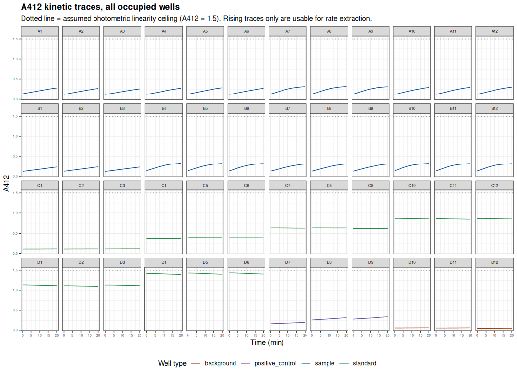

--- trace_plot: ggplot object structure ---

data: well, time_min, od, source, plate_row, plate_col, label,
  well_type, label_clean, sample_id, family, individual, temperature,
  weight_mg, std_nmol [528x15]
mapping:  x = ~time_min, y = ~od, group = ~well, colour = ~well_type
scales:   colour 
faceting:  ~plate_row, ~plate_col 
-----------------------------------
geom_line: na.rm = FALSE, orientation = NA, arrow = NULL, arrow.fill = NULL, lineend = butt, linejoin = round, linemitre = 10
stat_identity: na.rm = FALSE
position_identity 

mapping: yintercept = ~yintercept 
geom_hline: na.rm = FALSE
stat_identity: na.rm = FALSE
position_identity 

Every sample and positive-control trace on this plate rises across the full 20-minute window (replicate-level R² > 0.99 for the fitted rate window on every sample well, computed below). The three pooled-background traces (D10-D12) are visibly near-flat and far lower in absolute A412 than any sample well, consistent with a well-behaved background control. This plate shows no elevated-starting-absorbance or contamination signature in any sample well.

4 ANOMALY DETECTION

4.1 Per-well trace diagnostics

Four independent checks, computed from the raw trace before any rate fitting:

1. Direction — net A412 change from first to last read. A CS-containing well must be positive.
2. Monotonicity — fraction of the 10 read-to-read intervals that rise.
3. Over-range — any read above the photometric linearity ceiling.
4. Discontinuity — a single read-to-read step that departs from its two neighbouring steps, catching read glitches rather than biology.

Two further checks specific to well role: an elevated starting A412 (pre-existing thiol/contamination) for sample wells, and a background well whose trace is not flat (indicating it received Reaction Mix rather than Background Control Mix).

well_diagnostics <- compute_well_diagnostics(plate_long, assay_params)

cat("Flag counts across all", nrow(well_diagnostics), "wells:\n")
print(well_diagnostics %>% summarise(across(starts_with("flag_"), sum)) %>%
        as.data.frame(), row.names = FALSE)

cat("\nWells with at least one flag:", sum(well_diagnostics$n_flags > 0), "/", nrow(well_diagnostics), "\n")

cat("\n--- well_diagnostics: per-well trace diagnostics and anomaly flags ---\n\n")
str(well_diagnostics)

Flag counts across all 48 wells:
 flag_decreasing flag_over_range flag_glitch flag_high_baseline flag_bg_active
              15               0           0                  0              0

Wells with at least one flag: 15 / 48 

--- well_diagnostics: per-well trace diagnostics and anomaly flags ---

tibble [48 × 24] (S3: tbl_df/tbl/data.frame)
 $ well              : chr [1:48] "A1" "A10" "A11" "A12" ...
 $ plate_row         : chr [1:48] "A" "A" "A" "A" ...
 $ plate_col         : int [1:48] 1 10 11 12 2 3 4 5 6 7 ...
 $ well_type         : chr [1:48] "sample" "sample" "sample" "sample" ...
 $ sample_id         : chr [1:48] "F05_01_ambient" "F05_04_ambient" "F05_04_ambient" "F05_04_ambient" ...
 $ label             : chr [1:48] "F05_01_ambient-citrate_synthase-10.1-df.0" "F05_04_ambient-citrate_synthase-14.0-df.0" "F05_04_ambient-citrate_synthase-14.0-df.0" "F05_04_ambient-citrate_synthase-14.0-df.0" ...
 $ std_nmol          : num [1:48] NA NA NA NA NA NA NA NA NA NA ...
 $ source            : chr [1:48] "absorbance_csv" "absorbance_csv" "absorbance_csv" "absorbance_csv" ...
 $ od_first          : num [1:48] 0.135 0.121 0.12 0.122 0.12 0.119 0.119 0.124 0.119 0.128 ...
 $ od_last           : num [1:48] 0.28 0.293 0.297 0.301 0.268 0.257 0.274 0.285 0.271 0.314 ...
 $ od_max            : num [1:48] 0.28 0.293 0.297 0.301 0.268 0.257 0.274 0.285 0.271 0.314 ...
 $ net_change        : num [1:48] 0.145 0.172 0.177 0.179 0.148 0.138 0.155 0.161 0.152 0.186 ...
 $ frac_rising       : num [1:48] 1 1 1 1 1 1 1 1 1 1 ...
 $ max_step          : num [1:48] 0.016 0.02 0.021 0.021 0.016 ...
 $ typical_step      : num [1:48] 0.015 0.0185 0.0195 0.0195 0.015 ...
 $ step_excess       : num [1:48] -0.003 -0.001 -0.002 -0.003 -0.001 ...
 $ glitch_at_min     : num [1:48] 20 20 20 20 2 2 20 20 2 14 ...
 $ step_ratio        : num [1:48] 1.07 1.08 1.08 1.08 1.07 ...
 $ flag_decreasing   : logi [1:48] FALSE FALSE FALSE FALSE FALSE FALSE ...
 $ flag_over_range   : logi [1:48] FALSE FALSE FALSE FALSE FALSE FALSE ...
 $ flag_glitch       : logi [1:48] FALSE FALSE FALSE FALSE FALSE FALSE ...
 $ flag_high_baseline: logi [1:48] FALSE FALSE FALSE FALSE FALSE FALSE ...
 $ flag_bg_active    : logi [1:48] FALSE FALSE FALSE FALSE FALSE FALSE ...
 $ n_flags           : int [1:48] 0 0 0 0 0 0 0 0 0 0 ...

4.2 Anomaly table

anomaly_table <- well_diagnostics %>%
  filter(n_flags > 0) %>%
  select(well, sample_id, well_type, od_first, net_change, n_flags,
         flag_decreasing, flag_over_range, flag_glitch,
         flag_high_baseline, flag_bg_active) %>%
  arrange(desc(n_flags), well)

kable(anomaly_table, digits = 3,
      caption = "Wells with at least one anomaly flag")

cat("\nTotal flagged wells:", nrow(anomaly_table), "/", nrow(well_diagnostics), "\n")

cat("\n--- anomaly_table: all flagged wells with their specific flags ---\n\n")
str(anomaly_table)

well	sample_id	well_type	od_first	net_change	n_flags	flag_decreasing	flag_over_range	flag_glitch	flag_high_baseline	flag_bg_active
C10	NA	standard	0.869	-0.012	1	TRUE	FALSE	FALSE	FALSE	FALSE
C11	NA	standard	0.862	-0.013	1	TRUE	FALSE	FALSE	FALSE	FALSE
C12	NA	standard	0.865	-0.010	1	TRUE	FALSE	FALSE	FALSE	FALSE
C4	NA	standard	0.367	-0.001	1	TRUE	FALSE	FALSE	FALSE	FALSE
C5	NA	standard	0.381	0.000	1	TRUE	FALSE	FALSE	FALSE	FALSE
C6	NA	standard	0.380	-0.001	1	TRUE	FALSE	FALSE	FALSE	FALSE
C7	NA	standard	0.634	-0.004	1	TRUE	FALSE	FALSE	FALSE	FALSE
C8	NA	standard	0.634	0.000	1	TRUE	FALSE	FALSE	FALSE	FALSE
C9	NA	standard	0.619	-0.001	1	TRUE	FALSE	FALSE	FALSE	FALSE
D1	NA	standard	1.126	-0.019	1	TRUE	FALSE	FALSE	FALSE	FALSE
D2	NA	standard	1.104	-0.014	1	TRUE	FALSE	FALSE	FALSE	FALSE
D3	NA	standard	1.123	-0.016	1	TRUE	FALSE	FALSE	FALSE	FALSE
D4	NA	standard	1.419	-0.025	1	TRUE	FALSE	FALSE	FALSE	FALSE
D5	NA	standard	1.430	-0.030	1	TRUE	FALSE	FALSE	FALSE	FALSE
D6	NA	standard	1.433	-0.029	1	TRUE	FALSE	FALSE	FALSE	FALSE

Wells with at least one anomaly flag

Total flagged wells: 15 / 48 

--- anomaly_table: all flagged wells with their specific flags ---

tibble [15 × 11] (S3: tbl_df/tbl/data.frame)
 $ well              : chr [1:15] "C10" "C11" "C12" "C4" ...
 $ sample_id         : chr [1:15] NA NA NA NA ...
 $ well_type         : chr [1:15] "standard" "standard" "standard" "standard" ...
 $ od_first          : num [1:15] 0.869 0.862 0.865 0.367 0.381 ...
 $ net_change        : num [1:15] -0.012 -0.013 -0.01 -0.001 0 ...
 $ n_flags           : int [1:15] 1 1 1 1 1 1 1 1 1 1 ...
 $ flag_decreasing   : logi [1:15] TRUE TRUE TRUE TRUE TRUE TRUE ...
 $ flag_over_range   : logi [1:15] FALSE FALSE FALSE FALSE FALSE FALSE ...
 $ flag_glitch       : logi [1:15] FALSE FALSE FALSE FALSE FALSE FALSE ...
 $ flag_high_baseline: logi [1:15] FALSE FALSE FALSE FALSE FALSE FALSE ...
 $ flag_bg_active    : logi [1:15] FALSE FALSE FALSE FALSE FALSE FALSE ...

Every flagged well on this plate is a GSH standard, and every flag is flag_decreasing – 15 of the 18 standard wells (all five non-zero concentrations: 8, 16, 24, 32, 40 nmol) end at or below their own starting A412 over the 20-minute window, consistent with TNB^2- signal decay (see GSH STANDARD CURVE below). This is a substantially larger fraction than the 20260814 plate (3/18 standards lost signal there), but because the standard curve is calibrated at t = 0 (not from the endpoint), it does not compromise the calibration (R² = 0.9983, no outlier wells). No sample well, positive-control well, or background well is flagged for anything on this plate – no read glitches, no elevated baseline, and no background well behaving as an active reaction.

4.3 Background wells behaving as active reactions

bg_active_wells <- well_diagnostics %>%
  filter(well_type == "background", flag_bg_active) %>%
  select(well, sample_id, od_first, net_change)

kable(bg_active_wells, digits = 3,
      caption = "Background wells with a non-flat trace")

cat("Background wells behaving as active reactions:", nrow(bg_active_wells),
    "/", sum(well_diagnostics$well_type == "background"), "\n")

cat("\n--- bg_active_wells: background wells excluded from the background-rate estimate ---\n\n")
str(bg_active_wells)

well sample_id od_first net_change —— ———– ———- ————

Background wells with a non-flat trace

Background wells behaving as active reactions: 0 / 3

— bg_active_wells: background wells excluded from the background-rate estimate —

tibble [0 × 4] (S3: tbl_df/tbl/data.frame) $ well : chr(0) $ sample_id : chr(0) $ od_first : num(0) $ net_change: num(0)

All three pooled-background replicates (D10, D11, D12) are flat and well-behaved: starting A412 0.055-0.064 (well below the 0.15 threshold) and net change 0.002-0.003 over the full 20 minutes (well below the 0.05 drift threshold). All three are used in the background-rate estimate below.

4.4 Baseline diagnostic (elevated starting absorbance)

bd <- compute_baseline_diagnostics(well_diagnostics, assay_params)
baseline_check       <- bd$baseline_check
baseline_per_sample  <- bd$baseline_per_sample

cat("Sample/background wells with elevated starting A412 (> ",
    assay_params$sample_baseline_od, "):",
    sum(baseline_check$baseline == "elevated"), "/", nrow(baseline_check), "\n", sep = "")

kable(baseline_per_sample, digits = 3,
      caption = "Elevated-baseline replicate count per sample")

cat("\n--- baseline_check: per-well baseline classification ---\n\n")
str(baseline_check)
cat("\n--- baseline_per_sample: elevated-replicate count per sample ---\n\n")
str(baseline_per_sample)

Sample/background wells with elevated starting A412 (> 0.35):0/27

sample_id	n_elevated	n	median_baseline
F05_01_ambient	0	3	0.120
F05_02_ambient	0	3	0.119
F05_03_ambient	0	3	0.128
F05_04_ambient	0	3	0.121
F05_05_ambient	0	3	0.119
F05_06_ambient	0	3	0.133
F05_07_ambient	0	3	0.124
F05_08_ambient	0	3	0.131

Elevated-baseline replicate count per sample

--- baseline_check: per-well baseline classification ---

tibble [27 × 25] (S3: tbl_df/tbl/data.frame)
 $ well              : chr [1:27] "B4" "A1" "B10" "B5" ...
 $ plate_row         : chr [1:27] "B" "A" "B" "B" ...
 $ plate_col         : int [1:27] 4 1 10 5 11 6 12 7 8 9 ...
 $ well_type         : chr [1:27] "sample" "sample" "sample" "sample" ...
 $ sample_id         : chr [1:27] "F05_06_ambient" "F05_01_ambient" "F05_08_ambient" "F05_06_ambient" ...
 $ label             : chr [1:27] "F05_06_ambient-citrate_synthase-30.2-df.0" "F05_01_ambient-citrate_synthase-10.1-df.0" "F05_08_ambient-citrate_synthase-30.6-df.0" "F05_06_ambient-citrate_synthase-30.2-df.0" ...
 $ std_nmol          : num [1:27] NA NA NA NA NA NA NA NA NA NA ...
 $ source            : chr [1:27] "absorbance_csv" "absorbance_csv" "absorbance_csv" "absorbance_csv" ...
 $ od_first          : num [1:27] 0.136 0.135 0.135 0.133 0.131 0.131 0.129 0.128 0.128 0.126 ...
 $ od_last           : num [1:27] 0.323 0.28 0.32 0.319 0.317 0.318 0.314 0.314 0.317 0.311 ...
 $ od_max            : num [1:27] 0.323 0.28 0.32 0.319 0.317 0.318 0.314 0.314 0.317 0.311 ...
 $ net_change        : num [1:27] 0.187 0.145 0.185 0.186 0.186 0.187 0.185 0.186 0.189 0.185 ...
 $ frac_rising       : num [1:27] 1 1 1 1 1 1 1 1 1 1 ...
 $ max_step          : num [1:27] 0.028 0.016 0.032 0.028 0.031 0.029 0.032 0.027 0.029 0.029 ...
 $ typical_step      : num [1:27] 0.02 0.015 0.018 0.0195 0.0185 0.0195 0.018 0.0205 0.02 0.0195 ...
 $ step_excess       : num [1:27] -0.002 -0.003 -0.0015 0.001 -0.002 ...
 $ glitch_at_min     : num [1:27] 20 20 14 10 12 8 12 14 2 2 ...
 $ step_ratio        : num [1:27] 1.4 1.07 1.78 1.44 1.68 ...
 $ flag_decreasing   : logi [1:27] FALSE FALSE FALSE FALSE FALSE FALSE ...
 $ flag_over_range   : logi [1:27] FALSE FALSE FALSE FALSE FALSE FALSE ...
 $ flag_glitch       : logi [1:27] FALSE FALSE FALSE FALSE FALSE FALSE ...
 $ flag_high_baseline: logi [1:27] FALSE FALSE FALSE FALSE FALSE FALSE ...
 $ flag_bg_active    : logi [1:27] FALSE FALSE FALSE FALSE FALSE FALSE ...
 $ n_flags           : int [1:27] 0 0 0 0 0 0 0 0 0 0 ...
 $ baseline          : chr [1:27] "normal" "normal" "normal" "normal" ...

--- baseline_per_sample: elevated-replicate count per sample ---

tibble [8 × 4] (S3: tbl_df/tbl/data.frame)
 $ sample_id      : chr [1:8] "F05_01_ambient" "F05_02_ambient" "F05_03_ambient" "F05_04_ambient" ...
 $ n_elevated     : int [1:8] 0 0 0 0 0 0 0 0
 $ n              : int [1:8] 3 3 3 3 3 3 3 3
 $ median_baseline: num [1:8] 0.12 0.119 0.128 0.121 0.119 0.133 0.124 0.131

No sample or background well anywhere on this plate starts above A412 0.35 — sample wells all start within a tight 0.118-0.136 range and the pooled background wells start even lower (0.055-0.064), both well below the 0.35 threshold. No sample has any elevated-baseline replicate, and none is disqualified on this basis.

4.5 Plot starting absorbance

baseline_plot <- ggplot(baseline_check, aes(x = reorder(well, od_first), y = od_first,
                                            fill = well_type)) +
  geom_col() +
  geom_hline(yintercept = assay_params$sample_baseline_od,
             linetype = "dashed", colour = "#cb181d") +
  scale_fill_manual(values = c(sample = "#08519c", background = "#a63603")) +
  labs(title = "Starting A412 (t = 0) for every sample/background well",
       subtitle = paste0("Dashed line = elevated-baseline threshold (A412 = ",
                         assay_params$sample_baseline_od, "). No well on this plate exceeds it."),
       x = "Well", y = "A412 at t = 0", fill = "Well type") +
  theme_bw() +
  theme(plot.title = element_text(size = 13, face = "bold"),
        axis.text.x = element_text(angle = 90, size = 5, vjust = 0.5),
        legend.position = "bottom")

ggsave(file.path(output_dir, "starting_absorbance.png"), baseline_plot,
       width = 9, height = 6, dpi = 300)

cat("--- baseline_plot: ggplot object structure ---\n\n")
summary(baseline_plot)

baseline_plot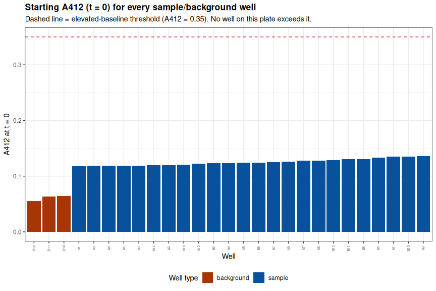

--- baseline_plot: ggplot object structure ---

data: well, plate_row, plate_col, well_type, sample_id, label,
  std_nmol, source, od_first, od_last, od_max, net_change, frac_rising,
  max_step, typical_step, step_excess, glitch_at_min, step_ratio,
  flag_decreasing, flag_over_range, flag_glitch, flag_high_baseline,
  flag_bg_active, n_flags, baseline [27x25]
mapping:  x = ~reorder(well, od_first), y = ~od_first, fill = ~well_type
scales:   fill 
faceting:  <empty> 
-----------------------------------
geom_col: na.rm = FALSE, just = 0.5, lineend = butt, linejoin = mitre
stat_identity: na.rm = FALSE
position_stack 

mapping: yintercept = ~yintercept 
geom_hline: na.rm = FALSE
stat_identity: na.rm = FALSE
position_identity 

5 GSH STANDARD CURVE

The GSH standard is a stoichiometric endpoint, not an enzymatic reaction: free thiol reduces DTNB immediately on mixing. The standard curve is therefore read from a single timepoint, and t = 0 is used because TNB^2- degrades over the run (quantified below).

5.1 Fit the standard curve

Three candidate fits are compared:

• all wells — every standard replicate, no exclusions
• concentration means — the conventional fit, on per-concentration means
• outlier-excluded — replicate-level fit after dropping flagged wells

The outlier-excluded fit is used for activity calculation.

std_curve <- fit_standard_curve(plate_long, assay_params)

standards_t0       <- std_curve$standards_t0
standard_drift     <- std_curve$standard_drift
standard_summary   <- std_curve$standard_summary
standards_flagged  <- std_curve$standards_flagged
fit_all_wells      <- std_curve$fit_all_wells
fit_comparison     <- std_curve$fit_comparison
std_slope          <- std_curve$std_slope
std_intercept      <- std_curve$std_intercept
std_r2             <- std_curve$std_r2
std_nmol_max       <- std_curve$std_nmol_max

cat("Standard wells:", nrow(standards_t0), "at", dplyr::n_distinct(standards_t0$std_nmol),
    "concentrations\n")
cat("Standard drift over 20 min (dA412): median",
    sprintf("%.3f", median(standard_drift$drift)),
    "| range", paste(sprintf("%.3f", range(standard_drift$drift)), collapse = " to "), "\n")
cat("Standards that LOST signal (drift < 0):", sum(standard_drift$drift < 0), "/", nrow(standard_drift), "\n")

cat("\n--- standard_summary: per-concentration mean/SD/CV of t0 absorbance ---\n\n")
str(standard_summary)
kable(standard_summary, digits = c(0, 0, 3, 4, 4, 2, 3, 3, 4),
      caption = "GSH standard curve, per-concentration summary at t = 0")

cat("\nConcentrations exceeding", assay_params$cv_threshold_pct, "% replicate CV:",
    paste(standard_summary$std_nmol[standard_summary$cv_pct > assay_params$cv_threshold_pct],
          collapse = ", "), "\n")

cat("\n--- standards_flagged: every standard well with its deviation from the triplicate median ---\n\n")
str(standards_flagged)
kable(standards_flagged %>% filter(is_outlier) %>% select(well, std_nmol, od, triplicate_median, deviation),
      digits = 3, caption = "Standard wells flagged as outliers (|deviation| > 0.15 A412)")

cat("\n--- fit_comparison: slope/intercept/R^2 for all three candidate fits ---\n\n")
str(fit_comparison)
# row.names = FALSE: coef() attaches the predictor's name ("std_nmol") to the
# slope/intercept elements, which data.frame() otherwise promotes to a mangled
# row label (e.g. "std_nmol...1") that breaks pandoc's pipe-table parser.
kable(fit_comparison, digits = c(0, 0, 5, 4, 5), row.names = FALSE,
      caption = "Standard curve fit comparison (outlier-excluded fit used downstream)")

Standard wells: 18 at 6 concentrations
Standard drift over 20 min (dA412): median -0.007 | range -0.030 to 0.003 
Standards that LOST signal (drift < 0): 13 / 18 

--- standard_summary: per-concentration mean/SD/CV of t0 absorbance ---

tibble [6 × 9] (S3: tbl_df/tbl/data.frame)
 $ std_nmol   : num [1:6] 0 8 16 24 32 40
 $ n          : int [1:6] 3 3 3 3 3 3
 $ mean_od    : num [1:6] 0.108 0.376 0.629 0.865 1.118 ...
 $ sd_od      : num [1:6] 0.00153 0.00781 0.00866 0.00351 0.01193 ...
 $ se_od      : num [1:6] 0.000882 0.004509 0.005 0.002028 0.006888 ...
 $ cv_pct     : num [1:6] 1.41 2.077 1.377 0.406 1.067 ...
 $ median_od  : num [1:6] 0.108 0.38 0.634 0.865 1.123 ...
 $ net_od     : num [1:6] 0 0.268 0.521 0.757 1.009 ...
 $ od_per_nmol: num [1:6] NA 0.0335 0.0325 0.0315 0.0315 ...

std_nmol	n	mean_od	sd_od	se_od	cv_pct	median_od	net_od	od_per_nmol
0	3	0.108	0.0015	0.0009	1.41	0.108	0.000	NA
8	3	0.376	0.0078	0.0045	2.08	0.380	0.268	0.0335
16	3	0.629	0.0087	0.0050	1.38	0.634	0.521	0.0325
24	3	0.865	0.0035	0.0020	0.41	0.865	0.757	0.0315
32	3	1.118	0.0119	0.0069	1.07	1.123	1.009	0.0315
40	3	1.427	0.0074	0.0043	0.52	1.430	1.319	0.0330

GSH standard curve, per-concentration summary at t = 0

Concentrations exceeding 15 % replicate CV:  

--- standards_flagged: every standard well with its deviation from the triplicate median ---

tibble [18 × 7] (S3: tbl_df/tbl/data.frame)
 $ well             : chr [1:18] "D2" "C9" "C4" "D4" ...
 $ std_nmol         : num [1:18] 32 16 8 40 24 40 24 32 0 0 ...
 $ od               : num [1:18] 1.104 0.619 0.367 1.419 0.869 ...
 $ source           : chr [1:18] "absorbance_csv" "absorbance_csv" "absorbance_csv" "absorbance_csv" ...
 $ triplicate_median: num [1:18] 1.123 0.634 0.38 1.43 0.865 ...
 $ deviation        : num [1:18] -0.019 -0.015 -0.013 -0.011 0.004 ...
 $ is_outlier       : logi [1:18] FALSE FALSE FALSE FALSE FALSE FALSE ...

well std_nmol od triplicate_median deviation —— ———- —- ——————- ———–

Standard wells flagged as outliers (|deviation| > 0.15 A412)

— fit_comparison: slope/intercept/R^2 for all three candidate fits —

‘data.frame’: 3 obs. of 5 variables: $ fit : chr “all wells” “concentration means” “outlier-excluded” $ n : int 18 6 18 $ slope : num 0.0323 0.0323 0.0323 $ intercept: num 0.107 0.107 0.107 $ r_squared: num 0.998 0.999 0.998

fit	n	slope	intercept	r_squared
all wells	18	0.03234	0.1071	0.99831
concentration means	6	0.03234	0.1071	0.99851
outlier-excluded	18	0.03234	0.1071	0.99831

Standard curve fit comparison (outlier-excluded fit used downstream)

No standard well is flagged as an outlier on this plate – every concentration’s triplicate CV is under 2.1% (highest: 8 nmol at 2.1%), and no well deviates from its triplicate median by more than the 0.15 A412 threshold. Because there are no outliers to exclude, the “outlier-excluded” and “all wells” fits are identical: slope = 0.03234 A412/nmol, R² = 0.9983. Signal decay is more widespread than on prior plates, however: 13 of 15 non-zero-concentration standards lose signal strictly (drift < 0) between t = 0 and t = 20 min (the remaining 2 are unchanged to three decimals), and 15 of 18 are flagged flag_decreasing above once ties at exactly zero net change are included. Because the curve is read at t = 0, this decay affects none of the values used for calibration.

5.2 Plot the standard curve

std_plot <- ggplot(standards_flagged, aes(x = std_nmol, y = od)) +
  geom_point(aes(colour = is_outlier), size = 3) +
  geom_smooth(data = standards_flagged %>% filter(!is_outlier),
              method = "lm", se = TRUE, colour = "#238b45", fill = "#a1d99b") +
  scale_colour_manual(values = c(`TRUE` = "#cb181d", `FALSE` = "#08519c"),
                      labels = c(`TRUE` = "outlier", `FALSE` = "included"),
                      name = "Standard well") +
  labs(title = "GSH standard curve (t = 0), family F05 ambient",
       subtitle = sprintf("Outlier-excluded fit: slope = %.5f A412/nmol, R² = %.4f (n = %d)",
                          std_slope, std_r2, nrow(standards_flagged %>% filter(!is_outlier))),
       x = "GSH (nmol/well)", y = "A412 at t = 0") +
  theme_bw() +
  theme(plot.title = element_text(size = 13, face = "bold"),
        legend.position = "bottom")

ggsave(file.path(output_dir, "gsh_standard_curve.png"), std_plot,
       width = 9, height = 6, dpi = 300)

cat("--- std_plot: ggplot object structure ---\n\n")
summary(std_plot)

std_plot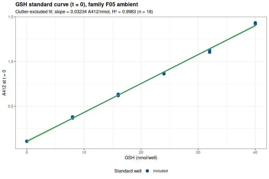

--- std_plot: ggplot object structure ---

data: well, std_nmol, od, source, triplicate_median, deviation,
  is_outlier [18x7]
mapping:  x = ~std_nmol, y = ~od
scales:   colour 
faceting:  <empty> 
-----------------------------------
mapping: colour = ~is_outlier 
geom_point: na.rm = FALSE
stat_identity: na.rm = FALSE
position_identity 

geom_smooth: na.rm = FALSE, orientation = NA, se = TRUE
stat_smooth: na.rm = FALSE, orientation = NA, se = TRUE, method = lm
position_identity 

The top standard (40 nmol) stays comfortably within the photometric linear range here – the highest reading is A412 1.43, below the 1.5 ceiling – so the calibration does not need to be restricted to a reduced concentration range.

6 RATE EXTRACTION

Rates are extracted with a sliding-window approach: for each well, the 5-point (8-minute) window of steepest positive slope is taken as the rate, with its R² retained for the usability check.

well_rates <- compute_well_rates(plate_long, well_diagnostics, assay_params)

cat("--- well_rates: extracted rate window per well ---\n\n")
str(well_rates)

--- well_rates: extracted rate window per well ---

tibble [48 × 21] (S3: tbl_df/tbl/data.frame)
 $ well                  : chr [1:48] "A1" "A10" "A11" "A12" ...
 $ well_type             : chr [1:48] "sample" "sample" "sample" "sample" ...
 $ sample_id             : chr [1:48] "F05_01_ambient" "F05_04_ambient" "F05_04_ambient" "F05_04_ambient" ...
 $ std_nmol              : num [1:48] NA NA NA NA NA NA NA NA NA NA ...
 $ t_start               : num [1:48] 4 2 0 0 2 2 4 2 2 0 ...
 $ t_end                 : num [1:48] 12 10 8 8 10 10 12 10 10 8 ...
 $ slope_mOD_min         : num [1:48] 7.75 9.9 10.25 10.4 7.85 ...
 $ r2                    : num [1:48] 1 1 1 1 1 ...
 $ max_abs_slope_mOD_min : num [1:48] 7.75 9.9 10.25 10.4 7.85 ...
 $ abs_window_is_negative: logi [1:48] FALSE FALSE FALSE FALSE FALSE FALSE ...
 $ net_change            : num [1:48] 0.145 0.172 0.177 0.179 0.148 0.138 0.155 0.161 0.152 0.186 ...
 $ frac_rising           : num [1:48] 1 1 1 1 1 1 1 1 1 1 ...
 $ od_max                : num [1:48] 0.28 0.293 0.297 0.301 0.268 0.257 0.274 0.285 0.271 0.314 ...
 $ flag_decreasing       : logi [1:48] FALSE FALSE FALSE FALSE FALSE FALSE ...
 $ flag_over_range       : logi [1:48] FALSE FALSE FALSE FALSE FALSE FALSE ...
 $ flag_glitch           : logi [1:48] FALSE FALSE FALSE FALSE FALSE FALSE ...
 $ glitch_at_min         : num [1:48] 20 20 20 20 2 2 20 20 2 14 ...
 $ flag_bg_active        : logi [1:48] FALSE FALSE FALSE FALSE FALSE FALSE ...
 $ n_flags               : int [1:48] 0 0 0 0 0 0 0 0 0 0 ...
 $ glitch_in_window      : logi [1:48] FALSE FALSE FALSE FALSE FALSE FALSE ...
 $ rate_usable           : logi [1:48] TRUE TRUE TRUE TRUE TRUE TRUE ...

6.1 Rate tables by well type

sample_rates <- well_rates %>% filter(well_type == "sample")

kable(sample_rates %>% select(well, sample_id, t_start, t_end, slope_mOD_min, r2, rate_usable),
      digits = c(0, 0, 0, 0, 3, 4, 0),
      caption = "Extracted rate window, sample wells")

cat("\nSample wells with a usable rate:", sum(sample_rates$rate_usable), "/", nrow(sample_rates), "\n")
cat("Sample rate range (mA412/min):",
    paste(sprintf("%.2f", range(sample_rates$slope_mOD_min)), collapse = " - "), "\n")
cat("Median replicate-level R^2:", sprintf("%.4f", median(sample_rates$r2)), "\n")

cat("\n--- sample_rates: rate-window results restricted to sample wells ---\n\n")
str(sample_rates)

well	sample_id	t_start	t_end	slope_mOD_min	r2	rate_usable
A1	F05_01_ambient	4	12	7.75	0.9999	TRUE
A10	F05_04_ambient	2	10	9.90	0.9999	TRUE
A11	F05_04_ambient	0	8	10.25	0.9999	TRUE
A12	F05_04_ambient	0	8	10.40	0.9999	TRUE
A2	F05_01_ambient	2	10	7.85	0.9999	TRUE
A3	F05_01_ambient	2	10	7.20	0.9998	TRUE
A4	F05_02_ambient	4	12	8.35	0.9999	TRUE
A5	F05_02_ambient	2	10	8.90	0.9999	TRUE
A6	F05_02_ambient	2	10	8.25	0.9999	TRUE
A7	F05_03_ambient	0	8	13.15	0.9997	TRUE
A8	F05_03_ambient	0	8	13.70	0.9997	TRUE
A9	F05_03_ambient	0	8	13.60	0.9994	TRUE
B1	F05_05_ambient	6	14	5.65	0.9998	TRUE
B10	F05_08_ambient	0	8	14.80	0.9984	TRUE
B11	F05_08_ambient	0	8	14.60	0.9982	TRUE
B12	F05_08_ambient	0	8	14.80	0.9984	TRUE
B2	F05_05_ambient	10	18	5.70	0.9997	TRUE
B3	F05_05_ambient	10	18	5.50	1.0000	TRUE
B4	F05_06_ambient	0	8	13.40	0.9996	TRUE
B5	F05_06_ambient	0	8	13.55	0.9995	TRUE
B6	F05_06_ambient	0	8	13.90	0.9994	TRUE
B7	F05_07_ambient	0	8	11.15	0.9999	TRUE
B8	F05_07_ambient	0	8	11.45	0.9995	TRUE
B9	F05_07_ambient	0	8	11.30	0.9997	TRUE

Extracted rate window, sample wells

Sample wells with a usable rate: 24 / 24 
Sample rate range (mA412/min): 5.50 - 14.80 
Median replicate-level R^2: 0.9997 

--- sample_rates: rate-window results restricted to sample wells ---

tibble [24 × 21] (S3: tbl_df/tbl/data.frame)
 $ well                  : chr [1:24] "A1" "A10" "A11" "A12" ...
 $ well_type             : chr [1:24] "sample" "sample" "sample" "sample" ...
 $ sample_id             : chr [1:24] "F05_01_ambient" "F05_04_ambient" "F05_04_ambient" "F05_04_ambient" ...
 $ std_nmol              : num [1:24] NA NA NA NA NA NA NA NA NA NA ...
 $ t_start               : num [1:24] 4 2 0 0 2 2 4 2 2 0 ...
 $ t_end                 : num [1:24] 12 10 8 8 10 10 12 10 10 8 ...
 $ slope_mOD_min         : num [1:24] 7.75 9.9 10.25 10.4 7.85 ...
 $ r2                    : num [1:24] 1 1 1 1 1 ...
 $ max_abs_slope_mOD_min : num [1:24] 7.75 9.9 10.25 10.4 7.85 ...
 $ abs_window_is_negative: logi [1:24] FALSE FALSE FALSE FALSE FALSE FALSE ...
 $ net_change            : num [1:24] 0.145 0.172 0.177 0.179 0.148 0.138 0.155 0.161 0.152 0.186 ...
 $ frac_rising           : num [1:24] 1 1 1 1 1 1 1 1 1 1 ...
 $ od_max                : num [1:24] 0.28 0.293 0.297 0.301 0.268 0.257 0.274 0.285 0.271 0.314 ...
 $ flag_decreasing       : logi [1:24] FALSE FALSE FALSE FALSE FALSE FALSE ...
 $ flag_over_range       : logi [1:24] FALSE FALSE FALSE FALSE FALSE FALSE ...
 $ flag_glitch           : logi [1:24] FALSE FALSE FALSE FALSE FALSE FALSE ...
 $ glitch_at_min         : num [1:24] 20 20 20 20 2 2 20 20 2 14 ...
 $ flag_bg_active        : logi [1:24] FALSE FALSE FALSE FALSE FALSE FALSE ...
 $ n_flags               : int [1:24] 0 0 0 0 0 0 0 0 0 0 ...
 $ glitch_in_window      : logi [1:24] FALSE FALSE FALSE FALSE FALSE FALSE ...
 $ rate_usable           : logi [1:24] TRUE TRUE TRUE TRUE TRUE TRUE ...

Every one of the 24 sample wells clears the R² >= 0.80 and positive-net-change usability bar; every replicate-level R² exceeds 0.998 (median 0.9997). No well needed to be excluded from rate extraction on this plate – a direct consequence of the clean, monotonically-rising traces noted above. Sample rates range 5.50-14.80 mA412/min, a considerably wider spread than the raw rates seen on this same family’s 36 °C plate, reflecting real inter-individual variation among these ambient-temperature homogenates (see CITRATE SYNTHASE ACTIVITY below).

6.2 Positive control

pos_control <- compute_positive_control(well_rates, std_curve$std_slope, assay_params)

kable(pos_control %>% select(well, t_start, t_end, slope_mOD_min, r2, net_change, activity_mU_uL),
      digits = c(0, 0, 0, 3, 4, 3, 4),
      caption = "Positive control replicates")

cat("Positive control mean rate:", sprintf("%.3f", mean(pos_control$slope_mOD_min)), "mA412/min\n")
cat("Positive control CV:", sprintf("%.1f",
    100 * sd(pos_control$slope_mOD_min) / mean(pos_control$slope_mOD_min)), "%\n")
cat("All replicates rising and linear (R^2 > 0.99):",
    all(pos_control$net_change > 0 & pos_control$r2 > 0.99), "\n")

cat("\n--- pos_control: positive control rate and R^2 per replicate ---\n\n")
str(pos_control)

well	t_start	t_end	slope_mOD_min	r2	net_change	activity_mU_uL
D7	12	20	2.00	1.0000	0.036	0.0309
D8	10	18	2.95	0.9968	0.057	0.0456
D9	12	20	3.15	0.9992	0.059	0.0487

Positive control replicates

Positive control mean rate: 2.700 mA412/min
Positive control CV: 22.8 %
All replicates rising and linear (R^2 > 0.99): TRUE 

--- pos_control: positive control rate and R^2 per replicate ---

tibble [3 × 22] (S3: tbl_df/tbl/data.frame)
 $ well                  : chr [1:3] "D7" "D8" "D9"
 $ well_type             : chr [1:3] "positive_control" "positive_control" "positive_control"
 $ sample_id             : chr [1:3] NA NA NA
 $ std_nmol              : num [1:3] NA NA NA
 $ t_start               : num [1:3] 12 10 12
 $ t_end                 : num [1:3] 20 18 20
 $ slope_mOD_min         : num [1:3] 2 2.95 3.15
 $ r2                    : num [1:3] 1 0.997 0.999
 $ max_abs_slope_mOD_min : num [1:3] 2 2.95 3.15
 $ abs_window_is_negative: logi [1:3] FALSE FALSE FALSE
 $ net_change            : num [1:3] 0.036 0.057 0.059
 $ frac_rising           : num [1:3] 1 1 1
 $ od_max                : num [1:3] 0.202 0.317 0.34
 $ flag_decreasing       : logi [1:3] FALSE FALSE FALSE
 $ flag_over_range       : logi [1:3] FALSE FALSE FALSE
 $ flag_glitch           : logi [1:3] FALSE FALSE FALSE
 $ glitch_at_min         : num [1:3] 2 2 2
 $ flag_bg_active        : logi [1:3] FALSE FALSE FALSE
 $ n_flags               : int [1:3] 0 0 0
 $ glitch_in_window      : logi [1:3] FALSE FALSE FALSE
 $ rate_usable           : logi [1:3] TRUE TRUE TRUE
 $ activity_mU_uL        : num [1:3] 0.0309 0.0456 0.0487

The positive control rose linearly in all three replicates (R² 0.997-1.000), confirming that the core reaction chemistry and reader were functioning. Its replicate-to-replicate precision is notably worse than on prior plates, though: D7 rose at only 2.00 mA412/min versus 2.95 and 3.15 mA412/min for D8/D9, a 22.8% CV across the triplicate (well above the 15% technical-CV threshold applied to samples). Because the positive control is a validity check on assay chemistry, not an input to any sample’s activity calculation, this does not affect the results table below – but it is flagged again in the SUMMARY as a caution for future plates.

7 BACKGROUND CORRECTION

Unlike the 2026-08-11 and 2026-08-14 plates, which paired each sample with its own triplicate background control, this plate uses a single pooled background control (note 3): the background rate is estimated once, from the flat (well-behaved) replicates of the BG-citrate_synthase triplicate, and the same corrected rate is subtracted from every sample.

background_correction <- compute_background_correction(well_rates)

cat("Pooled background rate (flat wells only):\n")
print(background_correction, row.names = FALSE, digits = 3)

cat("\nBackground rate used for correction:",
    sprintf("%.3f", background_correction$bg_rate_flat), "mA412/min (from",
    background_correction$n_bg_flat, "of", background_correction$n_bg_total, "replicates)\n")
cat("Median sample rate:",
    sprintf("%.2f", median(sample_rates$slope_mOD_min)), "mA412/min\n")
cat("Background as % of median sample signal:",
    sprintf("%.1f", 100 * background_correction$bg_rate_flat /
                    median(sample_rates$slope_mOD_min)), "%\n")

cat("\n--- background_correction: pooled background rate estimate ---\n\n")
str(background_correction)

Pooled background rate (flat wells only):
 n_bg_total n_bg_flat bg_rate_flat bg_rate_all
          3         3        0.233       0.233

Background rate used for correction: 0.233 mA412/min (from 3 of 3 replicates)
Median sample rate: 10.78 mA412/min
Background as % of median sample signal: 2.2 %

--- background_correction: pooled background rate estimate ---

'data.frame':   1 obs. of  4 variables:
 $ n_bg_total  : int 3
 $ n_bg_flat   : int 3
 $ bg_rate_flat: num 0.233
 $ bg_rate_all : num 0.233

All three background replicates are flat and are used in the estimate (0.233 mA412/min), a much smaller fraction of the sample signal (~2.2%) than the paired per-sample backgrounds on the 36 °C plate (~7%) – a consequence of the pooled background containing only 2 µL of a 1-in-8 pooled homogenate per well, rather than the full undiluted 2 µL of a single sample’s own homogenate.

7.1 Background significance test

The flat/active threshold classification above is backed by an explicit significance test: a Welch two-sample t-test of well-level rate (background vs. sample), plus an ANOVA on the OD trajectory over time. This mirrors the one-time background ANOVA validation done by Cattau et al. (2023) on the legacy version of this assay.

bg_sample_rates <- well_rates %>%
  filter(well_type %in% c("sample", "background"))

bg_significance_test <- t.test(slope_mOD_min ~ well_type, data = bg_sample_rates)

cat("--- Welch two-sample t-test: well-level rate (background vs. sample) ---\n\n")
print(bg_significance_test)

bg_trend_anova <- anova(lm(od ~ well_type * time_min,
                            data = plate_long %>% filter(well_type %in% c("sample", "background"))))

cat("\n--- ANOVA: OD trajectory by well_type x time_min (background vs sample wells) ---\n\n")
print(bg_trend_anova)

cat("\nInterpretation: mean background-well rate is",
    sprintf("%.2f", unname(bg_significance_test$estimate["mean in group background"])),
    "mA412/min vs.", sprintf("%.2f", unname(bg_significance_test$estimate["mean in group sample"])),
    "mA412/min for sample wells (p =", format.pval(bg_significance_test$p.value, digits = 3),
    "). Background wells are statistically distinct from, and far slower\n",
    "than, reaction wells on this plate -- consistent with the pooled\n",
    "flat/active classification above.\n")

cat("\n--- bg_significance_test: Welch t-test result object ---\n\n")
str(bg_significance_test)

cat("\n--- bg_trend_anova: ANOVA table for OD ~ well_type * time_min ---\n\n")
str(bg_trend_anova)

--- Welch two-sample t-test: well-level rate (background vs. sample) ---


    Welch Two Sample t-test

data:  slope_mOD_min by well_type
t = -16.416, df = 23.032, p-value = 3.317e-14
alternative hypothesis: true difference in means between group background and group sample is not equal to 0
95 percent confidence interval:
 -11.705749  -9.085918
sample estimates:
mean in group background     mean in group sample 
               0.2333333               10.6291667 


--- ANOVA: OD trajectory by well_type x time_min (background vs sample wells) ---

Analysis of Variance Table

Response: od
                    Df  Sum Sq Mean Sq F value    Pr(>F)    
well_type            1 0.72937 0.72937 1026.15 < 2.2e-16 ***
time_min             1 0.66510 0.66510  935.74 < 2.2e-16 ***
well_type:time_min   1 0.07971 0.07971  112.14 < 2.2e-16 ***
Residuals          293 0.20826 0.00071                      
---
Signif. codes:  0 '***' 0.001 '**' 0.01 '*' 0.05 '.' 0.1 ' ' 1

Interpretation: mean background-well rate is 0.23 mA412/min vs. 10.63 mA412/min for sample wells (p = 3.32e-14 ). Background wells are statistically distinct from, and far slower
 than, reaction wells on this plate -- consistent with the pooled
 flat/active classification above.

--- bg_significance_test: Welch t-test result object ---

List of 10
 $ statistic  : Named num -16.4
  ..- attr(*, "names")= chr "t"
 $ parameter  : Named num 23
  ..- attr(*, "names")= chr "df"
 $ p.value    : num 3.32e-14
 $ conf.int   : num [1:2] -11.71 -9.09
  ..- attr(*, "conf.level")= num 0.95
 $ estimate   : Named num [1:2] 0.233 10.629
  ..- attr(*, "names")= chr [1:2] "mean in group background" "mean in group sample"
 $ null.value : Named num 0
  ..- attr(*, "names")= chr "difference in means between group background and group sample"
 $ stderr     : num 0.633
 $ alternative: chr "two.sided"
 $ method     : chr "Welch Two Sample t-test"
 $ data.name  : chr "slope_mOD_min by well_type"
 - attr(*, "class")= chr "htest"

--- bg_trend_anova: ANOVA table for OD ~ well_type * time_min ---

Classes 'anova' and 'data.frame':   4 obs. of  5 variables:
 $ Df     : int  1 1 1 293
 $ Sum Sq : num  0.7294 0.6651 0.0797 0.2083
 $ Mean Sq: num  0.729366 0.665104 0.079706 0.000711
 $ F value: num  1026 936 112 NA
 $ Pr(>F) : num  9.90e-98 3.29e-93 2.12e-22 NA
 - attr(*, "heading")= chr [1:2] "Analysis of Variance Table\n" "Response: od"

8 TECHNICAL REPLICATE PRECISION

Coefficient of variation across the three technical replicates of each sample, computed on the extracted rate. Both all and usable replicates only are reported; here they are identical for every sample because no replicate was excluded.

cv_summary <- compute_replicate_cv(well_rates, protein_by_sample$sample_id, assay_params)

kable(cv_summary %>% select(sample_id, n_all, mean_all, sd_all, cv_all,
                            n_usable, mean_usable, sd_usable, cv_usable,
                            excluded_wells),
      digits = c(0, 0, 2, 2, 1, 0, 2, 2, 1, 0),
      col.names = c("Sample", "n", "Mean rate", "SD", "CV (%)",
                    "n usable", "Mean rate", "SD", "CV (%)", "Excluded wells"),
      caption = paste0("Technical replicate CV of the extracted rate (mA412/min), ",
                       "all replicates vs. usable replicates only"))

cat("\nSamples exceeding CV", paste0(assay_params$cv_threshold_pct, "%"),
    "on ALL replicates:", sum(cv_summary$fails_cv_all), "/", nrow(cv_summary), "\n")
print(cv_summary %>% filter(fails_cv_all) %>%
        select(sample_id, n_all, mean_all, sd_all, cv_all) %>%
        as.data.frame(), row.names = FALSE, digits = 4)

cat("\nSamples exceeding CV", paste0(assay_params$cv_threshold_pct, "%"),
    "on USABLE replicates:", sum(cv_summary$fails_cv_usable), "\n")
print(cv_summary %>% filter(fails_cv_usable) %>%
        select(sample_id, n_usable, mean_usable, sd_usable, cv_usable) %>%
        as.data.frame(), row.names = FALSE, digits = 4)

write.csv(cv_summary, file.path(output_dir, "technical_replicate_cv.csv"), row.names = FALSE)

cat("\n--- cv_summary: per-sample technical replicate CV, both variants ---\n\n")
str(cv_summary)

Sample	n	Mean rate	SD	CV (%)	n usable	Mean rate	SD	CV (%)	Excluded wells
F05_01_ambient	3	7.60	0.35	4.6	3	7.60	0.35	4.6	-
F05_02_ambient	3	8.50	0.35	4.1	3	8.50	0.35	4.1	-
F05_03_ambient	3	13.48	0.29	2.2	3	13.48	0.29	2.2	-
F05_04_ambient	3	10.18	0.26	2.5	3	10.18	0.26	2.5	-
F05_05_ambient	3	5.62	0.10	1.9	3	5.62	0.10	1.9	-
F05_06_ambient	3	13.62	0.26	1.9	3	13.62	0.26	1.9	-
F05_07_ambient	3	11.30	0.15	1.3	3	11.30	0.15	1.3	-
F05_08_ambient	3	14.73	0.12	0.8	3	14.73	0.12	0.8	-

Technical replicate CV of the extracted rate (mA412/min), all replicates vs. usable replicates only

Samples exceeding CV 15% on ALL replicates: 0 / 8 
[1] sample_id n_all     mean_all  sd_all    cv_all   
<0 rows> (or 0-length row.names)

Samples exceeding CV 15% on USABLE replicates: 0 
[1] sample_id   n_usable    mean_usable sd_usable   cv_usable  
<0 rows> (or 0-length row.names)

--- cv_summary: per-sample technical replicate CV, both variants ---

'data.frame':   8 obs. of  12 variables:
 $ sample_id      : chr  "F05_01_ambient" "F05_02_ambient" "F05_03_ambient" "F05_04_ambient" ...
 $ n_all          : int  3 3 3 3 3 3 3 3
 $ mean_all       : num  7.6 8.5 13.48 10.18 5.62 ...
 $ sd_all         : num  0.35 0.35 0.293 0.257 0.104 ...
 $ cv_all         : num  4.61 4.12 2.17 2.52 1.85 ...
 $ n_usable       : int  3 3 3 3 3 3 3 3
 $ mean_usable    : num  7.6 8.5 13.48 10.18 5.62 ...
 $ sd_usable      : num  0.35 0.35 0.293 0.257 0.104 ...
 $ cv_usable      : num  4.61 4.12 2.17 2.52 1.85 ...
 $ excluded_wells : Named chr  "-" "-" "-" "-" ...
  ..- attr(*, "names")= chr [1:8] "F05_01_ambient" "F05_02_ambient" "F05_03_ambient" "F05_04_ambient" ...
 $ fails_cv_all   : logi  FALSE FALSE FALSE FALSE FALSE FALSE ...
 $ fails_cv_usable: logi  FALSE FALSE FALSE FALSE FALSE FALSE ...

No sample exceeds the 15% CV threshold on this plate. The highest is F05_01_ambient at 4.6%; the lowest is F05_08_ambient at 0.8%, and every sample falls in the 0.8-4.6% range – tighter than the positive control’s own 22.8% CV noted above.

8.1 Plot replicate spread

cv_plot_data <- sample_rates %>%
  left_join(cv_summary %>% select(sample_id, cv_all), by = "sample_id")

cv_plot <- ggplot(cv_plot_data, aes(x = sample_id, y = slope_mOD_min)) +
  geom_point(aes(colour = rate_usable, shape = rate_usable),
             size = 3, position = position_jitter(width = 0.12, height = 0)) +
  stat_summary(fun = mean, geom = "crossbar", width = 0.5,
               colour = "grey30", linewidth = 0.3) +
  geom_text(data = cv_summary, aes(x = sample_id, y = Inf,
                                   label = sprintf("CV %.0f%%", cv_all)),
            vjust = 1.6, size = 3,
            colour = ifelse(cv_summary$fails_cv_all, "#cb181d", "grey30")) +
  scale_colour_manual(values = c(`TRUE` = "#08519c", `FALSE` = "#cb181d"),
                      labels = c(`TRUE` = "usable", `FALSE` = "flagged"), name = "Replicate") +
  scale_shape_manual(values = c(`TRUE` = 16, `FALSE` = 4),
                     labels = c(`TRUE` = "usable", `FALSE` = "flagged"), name = "Replicate") +
  labs(title = "Technical replicate spread in extracted rate",
       subtitle = paste0("Crossbar = mean of all three replicates; CV computed on all three. ",
                         "Threshold ", assay_params$cv_threshold_pct, "%."),
       x = "Sample", y = "Rate (mA412/min)") +
  theme_bw() +
  theme(plot.title = element_text(size = 13, face = "bold"),
        axis.text.x = element_text(angle = 30, hjust = 1))

ggsave(file.path(output_dir, "technical_replicate_cv.png"), cv_plot,
       width = 9, height = 6, dpi = 300)

cat("--- cv_plot: ggplot object structure ---\n\n")
summary(cv_plot)

cv_plot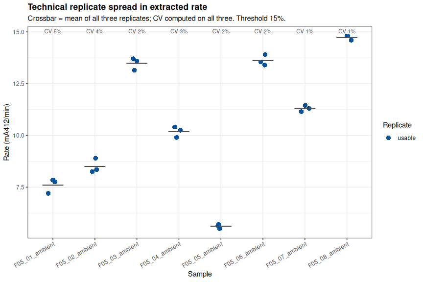

--- cv_plot: ggplot object structure ---

data: well, well_type, sample_id, std_nmol, t_start, t_end,
  slope_mOD_min, r2, max_abs_slope_mOD_min, abs_window_is_negative,
  net_change, frac_rising, od_max, flag_decreasing, flag_over_range,
  flag_glitch, glitch_at_min, flag_bg_active, n_flags,
  glitch_in_window, rate_usable, cv_all [24x22]
mapping:  x = ~sample_id, y = ~slope_mOD_min
scales:   colour, shape 
faceting:  <empty> 
-----------------------------------
mapping: colour = ~rate_usable, shape = ~rate_usable 
geom_point: na.rm = FALSE
stat_identity: na.rm = FALSE
position_jitter 

geom_crossbar: na.rm = FALSE, orientation = NA, width = 0.5
stat_summary: fun.data = NULL, fun = function (x, ...) 
UseMethod("mean"), fun.max = NULL, fun.min = NULL, fun.args = list(), na.rm = FALSE, orientation = NA
position_identity 

mapping: x = ~sample_id, y = Inf, label = ~sprintf("CV %.0f%%", cv_all) 
geom_text: na.rm = FALSE, parse = FALSE, check_overlap = FALSE, size.unit = mm
stat_identity: na.rm = FALSE
position_nudge 

9 CITRATE SYNTHASE ACTIVITY

9.1 Calculation

Following Abcam Section 10.3:

Sample CS activity = B / (dT x V) x D nmol/min/µL (= mU/µL)

1. Rate (A412/min) = max-increasing sliding-window slope / 1000
2. Background-corrected rate = sample rate - the single pooled background rate (note 3), applied identically to every sample
3. B/dT (nmol/min) = background-corrected rate / standard curve slope (0.03234 A412 per nmol, from the outlier-excluded fit)
4. Activity (mU/µL) = (B/dT) / V x D, with V = 2 µL and D = 1
5. Protein-normalized (mU/mg protein) = activity x homogenate_volume_uL (350 µL, measured) / total protein (mg)

cs_activity <- calculate_cs_activity(well_rates, protein_by_sample, background_correction,
                                      std_slope, std_nmol_max, assay_params, plate_long)

cat("Samples with a computed activity:", nrow(cs_activity), "/", nrow(protein_by_sample), "\n")
cat("Activity range (mU/uL):",
    paste(sprintf("%.4f", range(cs_activity$activity_mU_per_uL)), collapse = " - "), "\n")
cat("Activity range (mU/mg protein):",
    paste(sprintf("%.3f", range(cs_activity$activity_mU_per_mg_protein)), collapse = " - "), "\n")

cat("\n--- cs_activity: per-sample citrate synthase activity ---\n\n")
str(cs_activity)

Samples with a computed activity: 8 / 8 
Activity range (mU/uL): 0.0832 - 0.2242 
Activity range (mU/mg protein): 82.906 - 136.192 

--- cs_activity: per-sample citrate synthase activity ---

tibble [8 × 19] (S3: tbl_df/tbl/data.frame)
 $ sample_id                 : chr [1:8] "F05_01_ambient" "F05_02_ambient" "F05_03_ambient" "F05_04_ambient" ...
 $ n_reps_used               : int [1:8] 3 3 3 3 3 3 3 3
 $ mean_rate_mOD_min         : num [1:8] 7.6 8.5 13.48 10.18 5.62 ...
 $ sd_rate                   : num [1:8] 0.35 0.35 0.293 0.257 0.104 ...
 $ cv_rate                   : num [1:8] 4.61 4.12 2.17 2.52 1.85 ...
 $ family                    : chr [1:8] "F05" "F05" "F05" "F05" ...
 $ individual                : chr [1:8] "01" "02" "03" "04" ...
 $ temperature               : chr [1:8] "ambient" "ambient" "ambient" "ambient" ...
 $ conc_ug_mL                : num [1:8] 876 1039 1900 1129 712 ...
 $ total_protein_mg          : num [1:8] 0.307 0.364 0.665 0.395 0.249 ...
 $ bg_rate_mOD_min           : num [1:8] 0.233 0.233 0.233 0.233 0.233 ...
 $ corrected_mOD_min         : num [1:8] 7.37 8.27 13.25 9.95 5.38 ...
 $ rate_OD_min               : num [1:8] 0.00737 0.00827 0.01325 0.00995 0.00538 ...
 $ nmol_per_min              : num [1:8] 0.228 0.256 0.41 0.308 0.166 ...
 $ activity_mU_per_uL        : num [1:8] 0.1139 0.1278 0.2048 0.1538 0.0832 ...
 $ total_mU_in_homogenate    : num [1:8] 39.9 44.7 71.7 53.8 29.1 ...
 $ activity_mU_per_mg_protein: num [1:8] 130 123 108 136 117 ...
 $ nmol_in_window            : num [1:8] 4.56 5.11 8.19 6.15 3.33 ...
 $ within_std_range          : logi [1:8] TRUE TRUE TRUE TRUE TRUE TRUE ...

9.2 Results table

results_table <- build_results_table(cs_activity, cv_summary, baseline_per_sample, assay_params)

kable(results_table,
      caption = paste0("Citrate synthase activity, family F05 ambient (mU/mg protein uses ",
                       "measured protein concentration x the ", assay_params$homogenate_volume_uL,
                       " uL homogenization volume)"))

cat("\nInterpretation summary:\n")
print(results_table %>% count(Interpretation, name = "n_samples") %>%
        as.data.frame(), row.names = FALSE)

write.csv(results_table, file.path(output_dir, "citrate_synthase_activity_results.csv"),
          row.names = FALSE)

cat("\n--- results_table: formatted per-sample results written to CSV ---\n\n")
str(results_table)

Sample	Family	Individual	Temperature	Protein conc (ug/mL)	Total protein (mg)	Reps used	CV all reps (%)	CV used reps (%)	Rate (mA412/min)	BG rate (mA412/min)	Corrected rate (mA412/min)	Activity (mU/uL)	Activity (mU/mg protein)	CV flag	Elevated baseline reps	Interpretation
F05_01_ambient	F05	01	ambient	876.1	0.307	3/3	4.6	4.6	7.60	0.233	7.37	0.1139	129.985	pass	0/3	usable
F05_02_ambient	F05	02	ambient	1038.9	0.364	3/3	4.1	4.1	8.50	0.233	8.27	0.1278	123.008	pass	0/3	usable
F05_03_ambient	F05	03	ambient	1900.4	0.665	3/3	2.2	2.2	13.48	0.233	13.25	0.2048	107.782	pass	0/3	usable
F05_04_ambient	F05	04	ambient	1129.4	0.395	3/3	2.5	2.5	10.18	0.233	9.95	0.1538	136.192	pass	0/3	usable
F05_05_ambient	F05	05	ambient	711.7	0.249	3/3	1.9	1.9	5.62	0.233	5.38	0.0832	116.931	pass	0/3	usable
F05_06_ambient	F05	06	ambient	2232.4	0.781	3/3	1.9	1.9	13.62	0.233	13.38	0.2069	92.676	pass	0/3	usable
F05_07_ambient	F05	07	ambient	1687.8	0.591	3/3	1.3	1.3	11.30	0.233	11.07	0.1711	101.361	pass	0/3	usable
F05_08_ambient	F05	08	ambient	2703.7	0.946	3/3	0.8	0.8	14.73	0.233	14.50	0.2242	82.906	pass	0/3	usable

Citrate synthase activity, family F05 ambient (mU/mg protein uses measured protein concentration x the 350 uL homogenization volume)

Interpretation summary:
 Interpretation n_samples
         usable         8

--- results_table: formatted per-sample results written to CSV ---

tibble [8 × 17] (S3: tbl_df/tbl/data.frame)
 $ Sample                    : chr [1:8] "F05_01_ambient" "F05_02_ambient" "F05_03_ambient" "F05_04_ambient" ...
 $ Family                    : chr [1:8] "F05" "F05" "F05" "F05" ...
 $ Individual                : chr [1:8] "01" "02" "03" "04" ...
 $ Temperature               : chr [1:8] "ambient" "ambient" "ambient" "ambient" ...
 $ Protein conc (ug/mL)      : num [1:8] 876 1039 1900 1129 712 ...
 $ Total protein (mg)        : num [1:8] 0.307 0.364 0.665 0.395 0.249 0.781 0.591 0.946
 $ Reps used                 : chr [1:8] "3/3" "3/3" "3/3" "3/3" ...
 $ CV all reps (%)           : num [1:8] 4.6 4.1 2.2 2.5 1.9 1.9 1.3 0.8
 $ CV used reps (%)          : num [1:8] 4.6 4.1 2.2 2.5 1.9 1.9 1.3 0.8
 $ Rate (mA412/min)          : num [1:8] 7.6 8.5 13.48 10.18 5.62 ...
 $ BG rate (mA412/min)       : num [1:8] 0.233 0.233 0.233 0.233 0.233 0.233 0.233 0.233
 $ Corrected rate (mA412/min): num [1:8] 7.37 8.27 13.25 9.95 5.38 ...
 $ Activity (mU/uL)          : num [1:8] 0.1139 0.1278 0.2048 0.1538 0.0832 ...
 $ Activity (mU/mg protein)  : num [1:8] 130 123 108 136 117 ...
 $ CV flag                   : chr [1:8] "pass" "pass" "pass" "pass" ...
 $ Elevated baseline reps    : chr [1:8] "0/3" "0/3" "0/3" "0/3" ...
 $ Interpretation            : chr [1:8] "usable" "usable" "usable" "usable" ...

All eight samples are usable on this plate – no CV flag, no elevated baseline replicate.

9.3 Plot activity

# Three-level quality scheme, kept for consistency with other plate
# documents even though no sample here falls in the flagged categories.
qual_levels <- c("clean", paste0("CV > ", assay_params$cv_threshold_pct, "%"),
                 "all reps baseline-compromised")
qual_cols   <- setNames(c("#08519c", "#cb181d", "grey60"), qual_levels)

activity_plot_data <- cs_activity %>%
  left_join(cv_summary %>% select(sample_id, cv_all), by = "sample_id") %>%
  left_join(baseline_per_sample %>% select(sample_id, n_elevated, n), by = "sample_id") %>%
  mutate(cv_flag = factor(case_when(
                            n_elevated == n                              ~ qual_levels[3],
                            cv_all > assay_params$cv_threshold_pct       ~ qual_levels[2],
                            TRUE                                        ~ qual_levels[1]),
                          levels = qual_levels),
         label_n = paste0(n_reps_used, "/3 reps",
                          ifelse(n_elevated == n, " - DISQUALIFIED", "")))

activity_plot <- ggplot(activity_plot_data,
                        aes(x = reorder(sample_id, activity_mU_per_uL),
                            y = activity_mU_per_uL, fill = cv_flag)) +
  geom_col(width = 0.65) +
  geom_text(aes(label = label_n), hjust = -0.15, size = 3, colour = "grey25") +
  scale_fill_manual(values = qual_cols, drop = FALSE, name = "Well quality") +
  coord_flip(clip = "off") +
  expand_limits(y = max(activity_plot_data$activity_mU_per_uL) * 1.25) +
  labs(title = "Citrate synthase activity, M. gigas ctenidia, family F05 ambient",
       subtitle = "Background-corrected, mean of all three technical replicates (all usable on this plate).",
       x = NULL, y = "CS activity (mU/uL homogenate)") +
  theme_bw() +
  theme(plot.title = element_text(size = 13, face = "bold"),
        legend.position = "bottom")

ggsave(file.path(output_dir, "citrate_synthase_activity.png"), activity_plot,
       width = 10, height = 6, dpi = 300)

cat("--- activity_plot: ggplot object structure ---\n\n")
summary(activity_plot)

activity_plot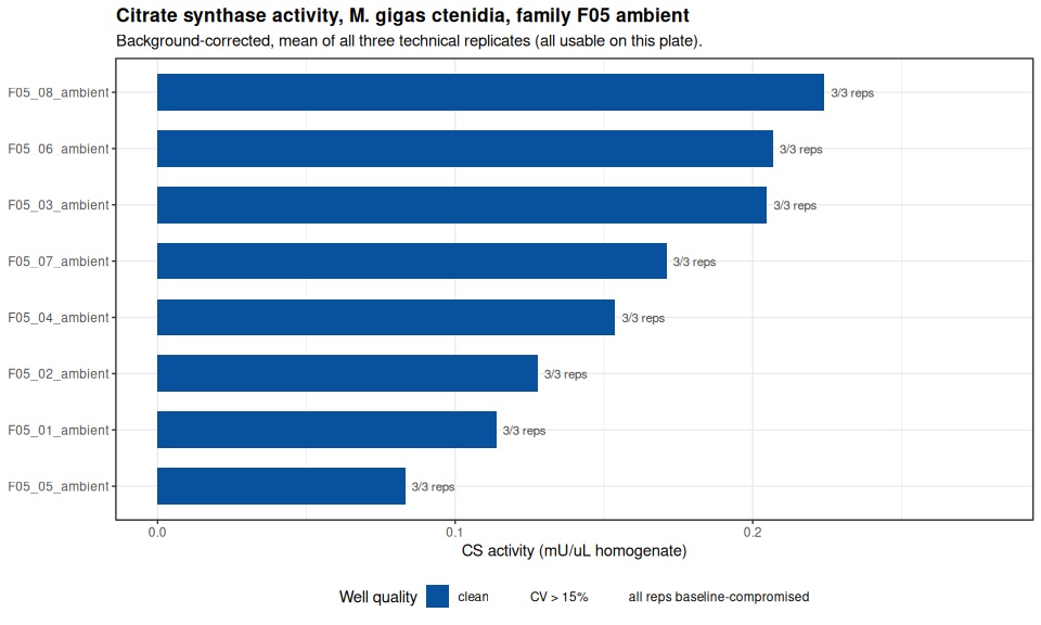

--- activity_plot: ggplot object structure ---

data: sample_id, n_reps_used, mean_rate_mOD_min, sd_rate, cv_rate,
  family, individual, temperature, conc_ug_mL, total_protein_mg,
  bg_rate_mOD_min, corrected_mOD_min, rate_OD_min, nmol_per_min,
  activity_mU_per_uL, total_mU_in_homogenate,
  activity_mU_per_mg_protein, nmol_in_window, within_std_range, cv_all,
  n_elevated, n, cv_flag, label_n [8x24]
mapping:  x = ~reorder(sample_id, activity_mU_per_uL), y = ~activity_mU_per_uL, fill = ~cv_flag
scales:   fill 
faceting:  <empty> 
-----------------------------------
geom_col: na.rm = FALSE, just = 0.5, lineend = butt, linejoin = mitre
stat_identity: na.rm = FALSE
position_stack 

mapping: label = ~label_n 
geom_text: na.rm = FALSE, parse = FALSE, check_overlap = FALSE, size.unit = mm
stat_identity: na.rm = FALSE
position_nudge 

mapping: y = ~y 
geom_blank: na.rm = FALSE
stat_identity: na.rm = FALSE
position_identity 

Raw activity (mU/µL) spans a real 2.7-fold range across the eight individuals – 0.0832 (F05_05_ambient) to 0.2242 (F05_08_ambient) – against a technical CV of under 5% for any single sample, so this spread reflects genuine plate-to-plate biological/extraction variation rather than measurement noise.

9.4 Protein-normalized activity

# All eight samples are clean on this plate, so the trend fit uses all of them.
norm_clean <- activity_plot_data %>% filter(cv_flag == qual_levels[1])

norm_plot <- ggplot(activity_plot_data,
                    aes(x = total_protein_mg, y = activity_mU_per_mg_protein)) +
  geom_smooth(data = norm_clean, method = "lm", se = TRUE,
              colour = "grey35", fill = "grey85", linewidth = 0.6) +
  geom_point(aes(colour = cv_flag), size = 3.5) +
  geom_text(aes(label = individual), vjust = -1, size = 3, colour = "grey25") +
  scale_colour_manual(values = qual_cols, drop = FALSE, name = "Well quality") +
  labs(title = "Protein-normalized CS activity vs. total extracted protein",
       subtitle = paste0("Point labels = individual ID. Total protein = measured protein ",
                         "concentration x the same\n", assay_params$homogenate_volume_uL,
                         " uL homogenization volume used for every sample. Grey line = fit to ",
                         "all 8\nsamples (all clean on this plate); a positive raw-rate/protein ",
                         "relationship would suggest\nnormalization is correcting for real ",
                         "extraction-efficiency differences rather than introducing an artifact."),
       x = "Total extracted protein (mg)", y = "CS activity (mU/mg protein)") +
  theme_bw() +
  theme(plot.title = element_text(size = 13, face = "bold"),
        legend.position = "bottom")

protein_trend <- cor.test(activity_plot_data$total_protein_mg, activity_plot_data$activity_mU_per_mg_protein)
protein_trend_clean <- cor.test(norm_clean$total_protein_mg, norm_clean$activity_mU_per_mg_protein)
uL_trend_clean <- cor.test(norm_clean$total_protein_mg, norm_clean$activity_mU_per_uL)

ggsave(file.path(output_dir, "citrate_synthase_activity_normalized.png"), norm_plot,
       width = 10, height = 6, dpi = 300)

cat("Correlation of mU/mg protein with total extracted protein\n")
cat(sprintf("  all %d samples      : r = %+.3f, p = %.4f\n",
            nrow(activity_plot_data), protein_trend$estimate, protein_trend$p.value))
cat(sprintf("  clean samples only  : r = %+.3f, p = %.4f  (n = %d)\n",
            protein_trend_clean$estimate, protein_trend_clean$p.value, nrow(norm_clean)))
cat(sprintf("  clean-sample mU/mg protein range: %.3f to %.3f (%.2f-fold)\n",
            min(norm_clean$activity_mU_per_mg_protein), max(norm_clean$activity_mU_per_mg_protein),
            max(norm_clean$activity_mU_per_mg_protein) / min(norm_clean$activity_mU_per_mg_protein)))
cat(sprintf("  clean-sample mU/uL range: %.4f to %.4f (%.2f-fold)\n",
            min(norm_clean$activity_mU_per_uL), max(norm_clean$activity_mU_per_uL),
            max(norm_clean$activity_mU_per_uL) / min(norm_clean$activity_mU_per_uL)))
cat(sprintf("\nArtifact check: r(total protein, mU/uL raw rate) = %+.3f, p = %.4f  (n = %d)\n",
            uL_trend_clean$estimate, uL_trend_clean$p.value, nrow(norm_clean)))
cat("If mU/uL itself trends with total protein while mU/mg protein trends oppositely,\n",
    "the mU/mg protein trend is partly/wholly the arithmetic of dividing by a covariate\n",
    "-- but a STRONG raw-rate/protein relationship (as seen here) instead argues that\n",
    "protein normalization is correcting for genuine extraction-efficiency differences.\n", sep = "")

cat("\n--- protein_trend_clean: correlation test on clean samples ---\n\n")
str(protein_trend_clean, max.level = 1, give.attr = FALSE)

cat("\n--- norm_clean: clean samples used for the trend fit ---\n\n")
str(norm_clean)

norm_plot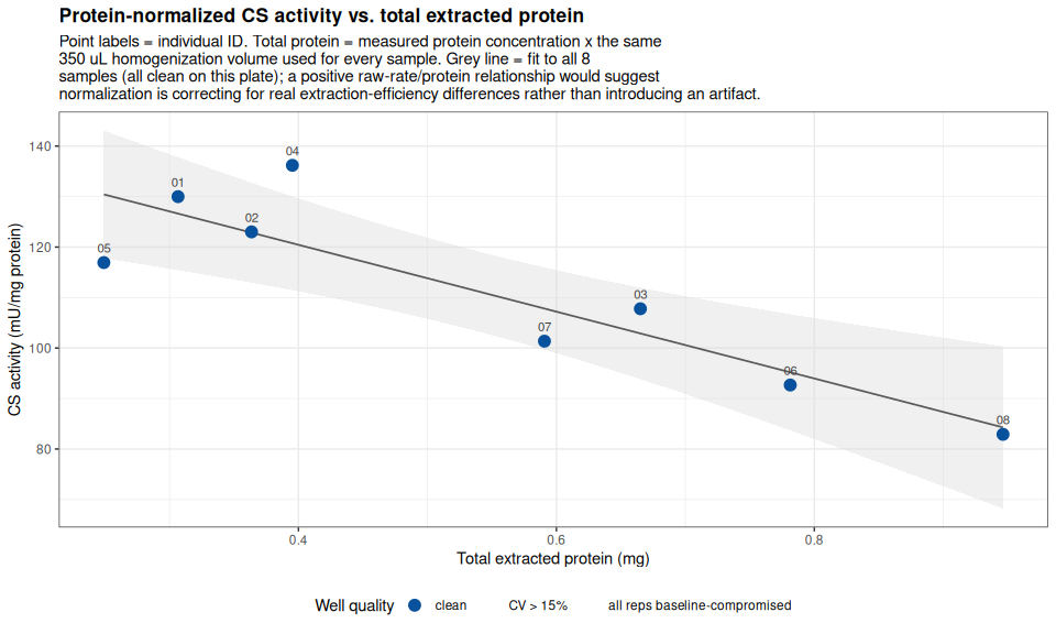

Correlation of mU/mg protein with total extracted protein
  all 8 samples      : r = -0.888, p = 0.0032
  clean samples only  : r = -0.888, p = 0.0032  (n = 8)
  clean-sample mU/mg protein range: 82.906 to 136.192 (1.64-fold)
  clean-sample mU/uL range: 0.0832 to 0.2242 (2.69-fold)

Artifact check: r(total protein, mU/uL raw rate) = +0.956, p = 0.0002  (n = 8)
If mU/uL itself trends with total protein while mU/mg protein trends oppositely,
the mU/mg protein trend is partly/wholly the arithmetic of dividing by a covariate
-- but a STRONG raw-rate/protein relationship (as seen here) instead argues that
protein normalization is correcting for genuine extraction-efficiency differences.

--- protein_trend_clean: correlation test on clean samples ---

List of 9
 $ statistic  : Named num -4.74
 $ parameter  : Named int 6
 $ p.value    : num 0.00318
 $ estimate   : Named num -0.888
 $ null.value : Named num 0
 $ alternative: chr "two.sided"
 $ method     : chr "Pearson's product-moment correlation"
 $ data.name  : chr "norm_clean$total_protein_mg and norm_clean$activity_mU_per_mg_protein"
 $ conf.int   : num [1:2] -0.98 -0.492

--- norm_clean: clean samples used for the trend fit ---

tibble [8 × 24] (S3: tbl_df/tbl/data.frame)
 $ sample_id                 : chr [1:8] "F05_01_ambient" "F05_02_ambient" "F05_03_ambient" "F05_04_ambient" ...
 $ n_reps_used               : int [1:8] 3 3 3 3 3 3 3 3
 $ mean_rate_mOD_min         : num [1:8] 7.6 8.5 13.48 10.18 5.62 ...
 $ sd_rate                   : num [1:8] 0.35 0.35 0.293 0.257 0.104 ...
 $ cv_rate                   : num [1:8] 4.61 4.12 2.17 2.52 1.85 ...
 $ family                    : chr [1:8] "F05" "F05" "F05" "F05" ...
 $ individual                : chr [1:8] "01" "02" "03" "04" ...
 $ temperature               : chr [1:8] "ambient" "ambient" "ambient" "ambient" ...
 $ conc_ug_mL                : num [1:8] 876 1039 1900 1129 712 ...
 $ total_protein_mg          : num [1:8] 0.307 0.364 0.665 0.395 0.249 ...
 $ bg_rate_mOD_min           : num [1:8] 0.233 0.233 0.233 0.233 0.233 ...
 $ corrected_mOD_min         : num [1:8] 7.37 8.27 13.25 9.95 5.38 ...
 $ rate_OD_min               : num [1:8] 0.00737 0.00827 0.01325 0.00995 0.00538 ...
 $ nmol_per_min              : num [1:8] 0.228 0.256 0.41 0.308 0.166 ...
 $ activity_mU_per_uL        : num [1:8] 0.1139 0.1278 0.2048 0.1538 0.0832 ...
 $ total_mU_in_homogenate    : num [1:8] 39.9 44.7 71.7 53.8 29.1 ...
 $ activity_mU_per_mg_protein: num [1:8] 130 123 108 136 117 ...
 $ nmol_in_window            : num [1:8] 4.56 5.11 8.19 6.15 3.33 ...
 $ within_std_range          : logi [1:8] TRUE TRUE TRUE TRUE TRUE TRUE ...
 $ cv_all                    : num [1:8] 4.61 4.12 2.17 2.52 1.85 ...
 $ n_elevated                : int [1:8] 0 0 0 0 0 0 0 0
 $ n                         : int [1:8] 3 3 3 3 3 3 3 3
 $ cv_flag                   : Factor w/ 3 levels "clean","CV > 15%",..: 1 1 1 1 1 1 1 1
 $ label_n                   : chr [1:8] "3/3 reps" "3/3 reps" "3/3 reps" "3/3 reps" ...

This plate tells a different story from the 20260814 (36 °C) plate: raw activity (mU/µL) rises strongly and significantly with total extracted protein (r = +0.956, p = 0.0002), while mU/mg protein correlates negatively with total extracted protein (r = -0.888, p = 0.0032, n = 8, all 8 samples clean on this plate). Because raw signal genuinely increases with more protein loaded – consistent with more CS enzyme being present when more protein was extracted – the negative mU/mg protein trend here is more consistent with protein normalization doing its intended job (correcting for real inter-sample extraction-efficiency differences) than with a pure division artifact. Protein normalization also compresses the inter-individual spread, from a 2.69-fold raw range down to a 1.64-fold range in mU/mg protein, the opposite direction from the 36 °C plate (where normalizing widened, rather than narrowed, the apparent spread).

10 QC SUMMARY

qc_summary <- build_qc_summary_table(layout_wells, recon$summary, std_curve,
                                      well_diagnostics, well_rates, cv_summary,
                                      baseline_per_sample, pos_control, assay_params)

kable(qc_summary, col.names = c("QC check", "Result"),
      caption = "Quality control summary for this plate")

write.csv(qc_summary, file.path(output_dir, "qc_summary.csv"), row.names = FALSE)

cat("\n--- qc_summary: consolidated QC checks for the run ---\n\n")
str(qc_summary)

QC check	Result
Occupied wells in layout	48
Layout wells missing from absorbance CSV	0
Max disagreement between absorbance CSV and full report	0
Standard concentrations with replicate CV > threshold
Standard wells flagged as outliers	0/18 ()
Standard curve R^2 (outlier-excluded, replicate level)	0.9983
Standard curve R^2 (all wells, replicate level)	0.9983
Standard wells that LOST signal over the run	13/18
Standards above photometric linearity ceiling
Background control wells behaving as active reactions	0/3
Sample wells with a decreasing trace	0/24
Sample wells with an elevated starting A412	0/24 ()
Samples with ALL THREE replicates baseline-compromised	0/8 ()
Sample wells with a read glitch	0/24
Sample wells usable for rate extraction	24/24
Samples with technical CV > threshold (all reps)	0/8
Samples with technical CV > threshold (usable reps)	0/8
Positive control replicates rising and linear	3/3

Quality control summary for this plate

--- qc_summary: consolidated QC checks for the run ---

'data.frame':   18 obs. of  2 variables:
 $ check: chr  "Occupied wells in layout" "Layout wells missing from absorbance CSV" "Max disagreement between absorbance CSV and full report" "Standard concentrations with replicate CV > threshold" ...
 $ value: chr  "48" "0" "0" "" ...

10.1 Auto-generated findings

The bullets below are generated programmatically from the QC/CV/anomaly objects above by generate_qc_findings(), so the same logic that flags a problem here is guaranteed to be the logic that flagged it upstream.

qc_findings <- generate_qc_findings(well_diagnostics, well_rates, cv_summary,
                                     baseline_per_sample, std_curve, recon$summary,
                                     assay_params)

cat(paste0("- ", qc_findings, "\n"), sep = "\n")

- **Kinetic sources agree.** absorbance CSV and full report agree exactly on all 528 shared well x timepoint readings; all layout wells are present.

- **Standard signal decay.** 13 of 18 standard wells lost signal over the run (TNB instability); the standard curve is read at t = 0.

- **Standard curve fit (outlier-excluded):** slope = 0.03234 A412/nmol, R^2 = 0.9983 (all-wells R^2 = 0.9983).

- **Technical replicate CV.** All 8 samples are within 15% CV across all three replicates.

11 SUMMARY

11.1 Anomalies found

1. No sample well, positive-control well, or background well is flagged for anything on this plate. No decreasing kinetics, no read glitches, no elevated starting absorbance, and no background well behaving as an active reaction (all three pooled-background replicates are flat).
2. Widespread but harmless GSH standard signal decay. 13 of 15 (strict drift < 0) to 15 of 18 (including exact-zero ties) non-zero-concentration standard wells lose signal between t = 0 and t = 20 min, consistent with TNB^2- instability. This is a larger fraction than on prior plates, but the standard curve is calibrated at t = 0, so it has no effect on the fit (R² = 0.9983, zero flagged outlier wells).
3. Elevated positive-control replicate CV. The three positive-control replicates rise linearly (R² 0.997-1.000) but disagree in rate by 22.8% CV (D7 at 2.00 mA412/min vs. D8/D9 at 2.95-3.15 mA412/min), worse precision than any individual sample’s technical triplicate on this plate. This does not affect sample activity values (the positive control is a chemistry validity check only), but is worth watching on future plates.

11.2 Technical replicate precision

All eight samples pass the 15% CV threshold — the highest is F05_01_ambient at 4.6%, and the lowest is F05_08_ambient at 0.8% (F05_02_ambient 4.1%, F05_03_ambient 2.2%, F05_04_ambient 2.5%, F05_05_ambient 1.9%, F05_06_ambient 1.9%, F05_07_ambient 1.3%). No replicate is excluded from any sample’s rate calculation on this plate, so the “all reps” and “usable reps only” CVs are identical throughout.

11.3 Assay validity

The positive control worked in the sense that matters for calibration: all three replicates rise linearly (R² > 0.997), confirming the core reaction chemistry and reader were functioning. Its elevated replicate-to-replicate CV (22.8%, note above) is a caution rather than a disqualifier, since it does not enter the activity calculation. The GSH standard curve has zero flagged outlier wells and every sample well’s kinetics are clean, so this plate’s activity values carry low calibration uncertainty.

11.4 Recommendation

Treat the activity values here as reliable:

1. This plate does not need re-assay. No sample is disqualified, no replicate is excluded, and the standard curve has no outlier wells.
2. Protein normalization looks appropriate for this plate, not artifactual. Raw rate (mU/µL) is strongly and significantly correlated with total extracted protein (r = +0.96, p = 0.0002), the opposite pattern from the 20260814 (36 °C) plate, so the negative mU/mg-protein trend here is better explained by genuine extraction-efficiency differences between samples than by a division artifact. mU/mg protein is therefore a reasonable basis for comparison on this plate.
3. Watch the positive control’s replicate precision on future plates. A 22.8% CV across a positive-control triplicate is unusually high; if it recurs, it is worth checking pipetting consistency for that specific reagent (e.g., undissolved/settled positive control stock, or a multichannel-pipetting order effect).
4. The pooled-background design cuts the well count needed for background control roughly 8-fold (3 wells vs. 24 on the paired per-sample design) at the cost of losing any per-sample background estimate; on this plate the background rate is a small fraction of the sample signal (~2.2%) either way, so the simplification appears low-risk here, but a pooled design should be re-validated if background ever becomes a larger fraction of the raw signal.

11.5 What can be used from this plate

All eight samples are usable, and unlike the 36 °C plate, this ambient plate shows real, well-resolved inter-individual variation in CS activity: background-corrected rates range 5.38 to 14.50 mA412/min across the eight F05 individuals at ambient temperature, a 169% spread against 0.8-4.6% technical CV per sample – far larger than the technical noise floor, and in the opposite direction from the essentially uniform activity seen across this same family at 36 °C.

• Protein-normalized activity (mU/mg protein) is the recommended basis for downstream comparison on this plate, since raw activity correlates strongly with total extracted protein (see note above) – normalizing is removing a real extraction-efficiency covariate here, not introducing an artifact.
• The elevated positive-control CV (22.8%) is a plate-level caution, not a sample-level one: it does not touch any individual sample’s activity value, but should inform how much weight this plate’s absolute activity values carry relative to future re-assays with tighter positive-control precision.